Improved Curvature Estimation for Computer-aided Detection of Colonic Polyps in CT Colonography

Rationale and Objectives

Current schemes for computer-aided detection (CAD) of colon polyps usually use kernel methods to perform curvature-based shape analysis. However, kernel methods may deliver spurious curvature estimations if the kernel contains two surfaces, because of the vanished gradient magnitudes. The aim of this study was to use the Knutsson mapping method to deal with the difficulty of providing better curvature estimations and to assess the impact of improved curvature estimation on the performance of CAD schemes.

Materials and Methods

The new method was compared to two widely used kernel methods in terms of the performance of two stages of CAD: initial detection and true-positive and false-positive classification. The evaluation was conducted on a database of 130 computed tomographic scans from 67 patients. In these patient scans, there were 104 clinically significant polyps and masses >5 mm.

Results

In the initial detection stage, the detection sensitivity of the three methods was comparable. In the classification stage, at a 90% sensitivity level on the basis of the input of this step, the new technique yielded 3.15 false-positive results per scan, demonstrating reductions in false-positive findings of 30.2% ( P < .01) and 27.9% ( P < .01) compared to the two kernel methods.

Conclusions

The new method can benefit CAD schemes with reduced false-positive rates, without sacrificing detection sensitivity.

According to recent statistics from the American Cancer Society , colorectal cancer is the third most common cause of both cancer deaths and new cancer cases in both men and women in the United States. Most colon cancers start from benign polyps, and the transformation from benignity to malignance often takes 5 to 10 years. Therefore, early detection and removal of colonic polyps prior to their malignant transformation can effectively decrease the incidence of colon cancer . Colon polyps are not commonly associated with any symptoms. Therefore, adequate time interval screening is recommended for people aged > 50 years by the American Cancer Society . As a new minimally invasive screening technique, computed tomographic colonography (CTC) or computed tomography–based virtual colonoscopy has shown several advantages over the traditional optical colonoscopy . To improve the performance of CTC in detecting polyps, computer-aided detection (CAD) has shown the potential to assist physicians in finding and analyzing polyps in the colon .

In most currently available CAD systems in CTC, principal curvatures, estimated through kernel methods , and principal curvature–related measures, such as mean curvatures, Gaussian curvatures, sphericity ratio, shape index, and curvedness, are widely used to characterize the shapes of colon polyps . However, when a kernel contains two surfaces (as happens for thin slab objects such as colonic folds and spherical objects such as polyps), spurious estimations of curvatures are frequently observed, indicating false high curvature . This is due to the discontinuity at thin structures, where the curvatures are discontinuous because of the diminished gradient magnitude. Fortunately, this discontinuity problem can be solved using Knutsson mapping , which maps a discontinuous orientation field into a continuous one. In this study, we adapted the Knutsson mapping technique to accurately estimate principal curvatures and explored the possible benefits of such improved curvature estimation for CAD performance in CTC. Evaluation of the new technique using both phantom experiments and patient studies demonstrated a noticeable reduction in the false-positive (FP) rate for CAD of colonic polyps compared to two current kernel methods.

Materials and methods

Methods

Get Radiology Tree app to read full this article<

Kernel methods for estimation of principal curvatures

Get Radiology Tree app to read full this article<

kT=k×N, k

T

=

k

×

N

,

where k is the curvature vector of the concerned curve at that point, and N is the unit normal at that point on the surface. Nonsingular curves that have the same tangent vector T will have the same curvature kT . Among all possible tangent vectors, the maximum and minimum values of kT at that point are called the principal curvatures, k 1 and k 2 , and the directions of the corresponding tangent vectors are called principal directions.

Get Radiology Tree app to read full this article<

Get Radiology Tree app to read full this article<

kT=−(TtΩHT)/∥g∥, k

T

=

−

(

T

t

Ω

H

T

)

/

‖

g

‖

,

where Ω H is the Hessian matrix of the volume image, and g is the gradient vector (the normal vector). The resulted principal curvatures and directions were expressed as functions of the first and second derivatives of the image. In the kernel method developed by Thirion and Gourdon , denoted as KM 2 in the following text, equation (1) was rewritten as

k1,2=H±Δ−−√withΔ=H2−K, k

1

,

2

=

H

±

Δ

with

Δ

=

H

2

−

K

,

where H = ( k 1 + k 2 ) and K = k 1 k 2 are the mean and Gaussian curvatures. They can be computed using the following formulas:

H=12∥g∥3[I2x(Iyy+Izz)−2IyIzIyz+I2y(Ixx+Izz)−2IxIzIxz+I2z(Ixx+Iyy)−2IxIyIxy, H

=

1

2

‖

g

‖

3

[

I

x

2

(

I

y

y

+

I

z

z

)

−

2

I

y

I

z

I

y

z

+

I

y

2

(

I

x

x

+

I

z

z

)

−

2

I

x

I

z

I

x

z

+

I

z

2

(

I

x

x

+

I

y

y

)

−

2

I

x

I

y

I

x

y

,

K=1∥g∥4[I2x(IyyIzz+I2yz)−2IyIz(IxzIxy−IxxIyz)+I2y(IxxIzz+I2xz)−2IxIz(IyzIxy−IyyIxz)+I2z(IxxIyy+I2xy)−2IxIy(IxzIyz−IzzIxy). K

=

1

‖

g

‖

4

[

I

x

2

(

I

y

y

I

z

z

+

I

y

z

2

)

−

2

I

y

I

z

(

I

x

z

I

x

y

−

I

x

x

I

y

z

)

+

I

y

2

(

I

x

x

I

z

z

+

I

x

z

2

)

−

2

I

x

I

z

(

I

y

z

I

x

y

−

I

y

y

I

x

z

)

+

I

z

2

(

I

x

x

I

y

y

+

I

x

y

2

)

−

2

I

x

I

y

(

I

x

z

I

y

z

−

I

z

z

I

x

y

)

.

Get Radiology Tree app to read full this article<

Get Radiology Tree app to read full this article<

Knutsson mapping

Get Radiology Tree app to read full this article<

Get Radiology Tree app to read full this article<

kT=∥∇TN∥. k

T

=

‖

∇

T

N

‖

.

Get Radiology Tree app to read full this article<

Get Radiology Tree app to read full this article<

Get Radiology Tree app to read full this article<

|k1,2|=12√∥∇e2,3M(e1)∥=12√∥∥∑3n=1∂Mij∂xnen2,3∥∥, |

k

1

,

2

|

=

1

2

‖

∇

e

2

,

3

M

(

e

1

)

‖

=

1

2

‖

∑

n

=

1

3

∂

M

i

j

∂

x

n

e

2

,

3

n

‖

,

where M ij is the element of the second-order tensor M ( e 1 ), and x n a coordinate. The norm is the Fröbenius norm ∥M∥2=∑i,jm2ij ‖

M

‖

2

=

∑

i

,

j

m

i

j

2 . To be clearer, equation 7 can be laid out as

|k1,2|=12√∥∥∑3n=1∂Mij∂xnen2,3∥∥=12√∥∥∂Mij∂xex2,3+∂Mij∂yey2,3+∂Mij∂zez2,3∥∥, |

k

1

,

2

|

=

1

2

‖

∑

n

=

1

3

∂

M

i

j

∂

x

n

e

2

,

3

n

‖

=

1

2

‖

∂

M

i

j

∂

x

e

2

,

3

x

+

∂

M

i

j

∂

y

e

2

,

3

y

+

∂

M

i

j

∂

z

e

2

,

3

z

‖

,

where ex2,3 e

2

,

3

x , ey2,3 e

2

,

3

y , and ez2,3 e

2

,

3

z represent the coordinates of the vectors e 2 and e 3 . Another scale, σ k , is involved for evaluating first-order derivative ∇Mij=(∂Mij∂x,∂Mij∂y,∂Mij∂z)=Mij×∇G(σk) ∇

M

i

j

=

(

∂

M

i

j

∂

x

,

∂

M

i

j

∂

y

,

∂

M

i

j

∂

z

)

=

M

i

j

×

∇

G

(

σ

k

) through the Gaussian derivative ∇G(σk) ∇

G

(

σ

k

) . The sign of the curvatures is the negative of the sign of Tt Ω H T , where Ω H represents the Hessian matrix.

Get Radiology Tree app to read full this article<

Get Radiology Tree app to read full this article<

Experimental Design

CAD pipeline

Get Radiology Tree app to read full this article<

Get Radiology Tree app to read full this article<

Get Radiology Tree app to read full this article<

Get Radiology Tree app to read full this article<

Method parameter configuration

Get Radiology Tree app to read full this article<

Table 1

Parameters Involved in Stage 2 of the Computer-Aided Diagnosis (CAD) Pipeline

Method Parameters Kernel method 1 α 1 , α 2 Kernel method 2 σ 1 , σ 2 Knutsson mapping kernel method σ g , σ T , σ k

Get Radiology Tree app to read full this article<

Get Radiology Tree app to read full this article<

Get Radiology Tree app to read full this article<

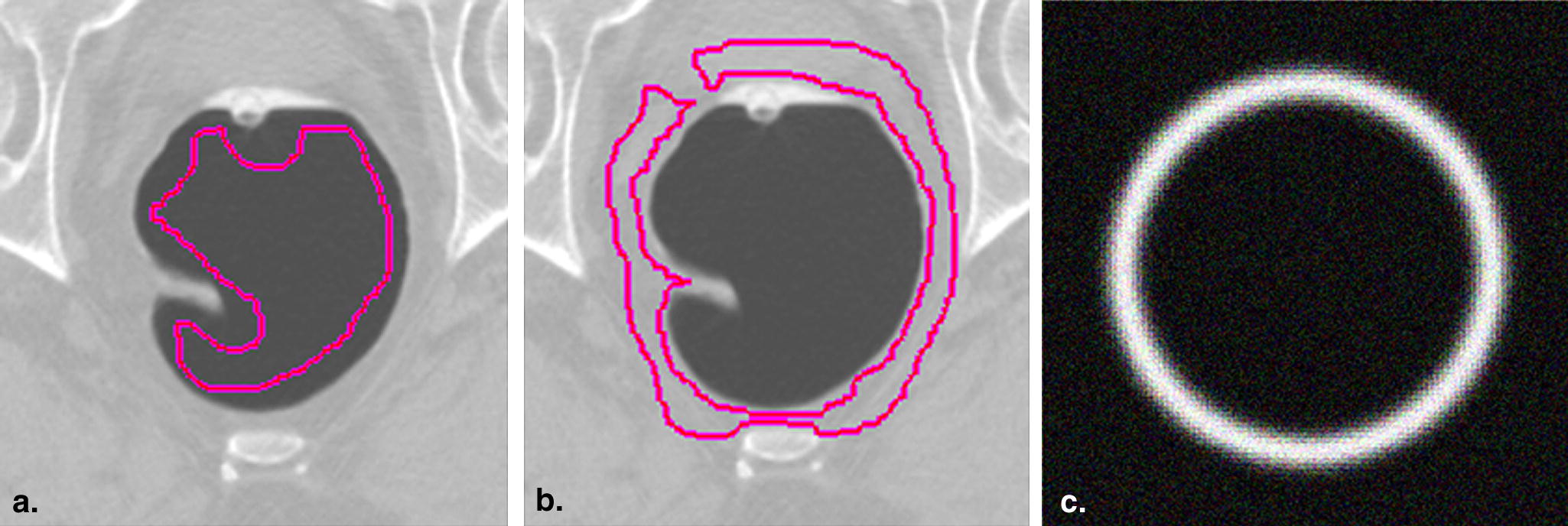
Table 2

Means and Standard Deviations of Regions of Interest in Colon Lumen and Tissue Adjacent to Colon Wall

Mean Standard Deviation Lumen (Hounsfield units) 41.54 23.64 Adjacent tissue (Hounsfield units) 937.81 38.77

Get Radiology Tree app to read full this article<

Get Radiology Tree app to read full this article<

Table 3

Size Distribution of the Polyps

Size (mm) n (%) 6–9 118 (56.7) 10–30 82 (39.4) >30 8 (3.8)

Get Radiology Tree app to read full this article<

CTC Database

Get Radiology Tree app to read full this article<

Table 4

Shape Distribution of the Polyps

Shape n (%) Sessile 103 (49.5) Pedunculated 92 (44.2) Flat 13 (6.3)

Get Radiology Tree app to read full this article<

Performance evaluation for patient studies

Get Radiology Tree app to read full this article<

Get Radiology Tree app to read full this article<

Get Radiology Tree app to read full this article<

Results

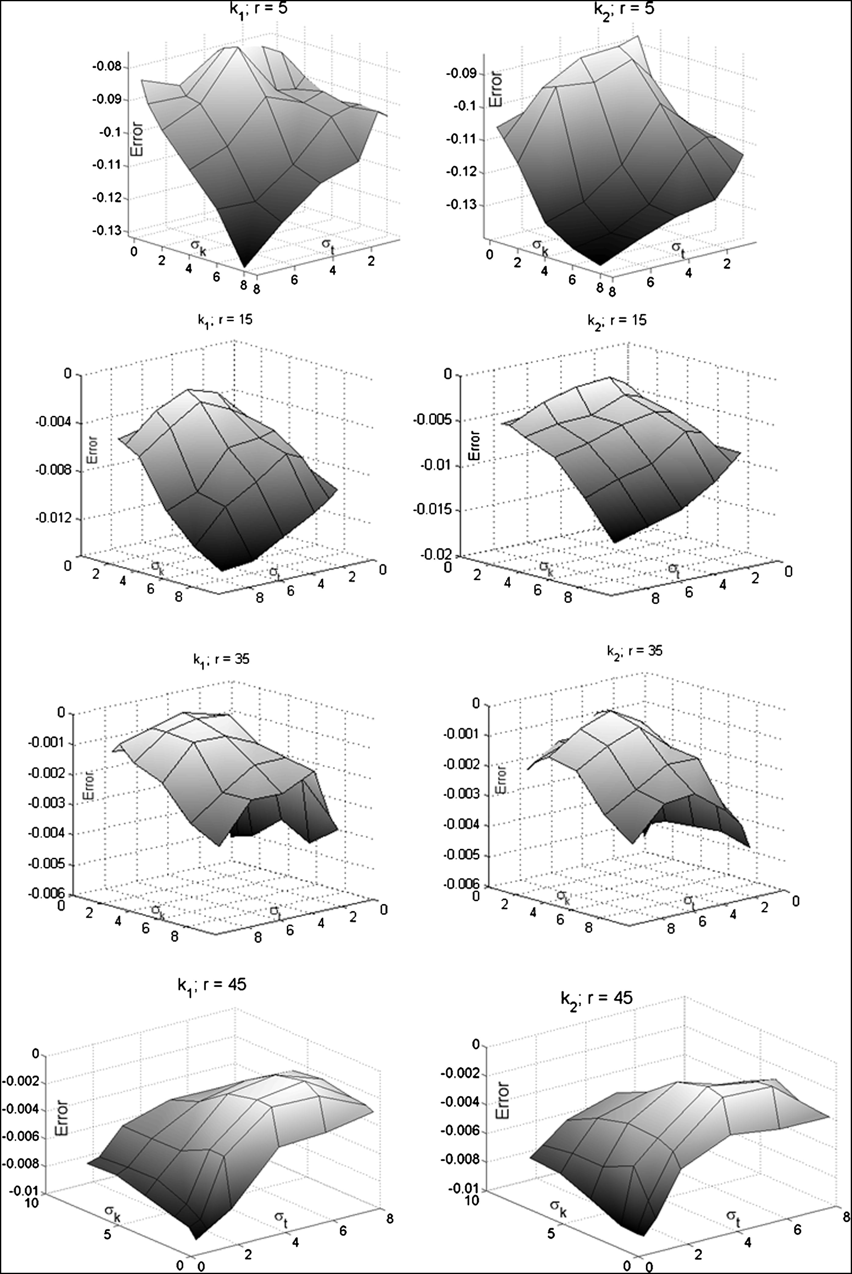
Phantom Study

Get Radiology Tree app to read full this article<

![Figure 3, Plots of error (vertical axis) (ie,

k 1,2

− k theory ) according to objects with various sizes ( r = 5, 15, 35, and 45 from top to bottom rows) and various values of σ T and σ k (two horizontal axes) with the Knutsson mapping kernel method. The left and right columns indicate the errors of k 1 and k 2 .](https://storage.googleapis.com/dl.dentistrykey.com/clinical/ImprovedCurvatureEstimationforComputeraidedDetectionofColonicPolypsinCTColonography/2_1s20S1076633211002066.jpg)

Get Radiology Tree app to read full this article<

Get Radiology Tree app to read full this article<

Table 5

Statistics of | k 1 | and | k 2 | Resulting From the Three Methods

KM 1 KM 2 KM M Mean Variance Mean Variance Mean Variance_r_ = 14 (| k 1 | = | k 2 | ≈ 0.0714) k 1 | 2.24 1.01 1.88 0.86 0.0684 0.000210 k 2 | 3.15 1.15 2.87 0.97 0.0672 0.00722r = 15 (| k 1 | = | k 2 | ≈ 0.0667) k 1 | 23.04 302 21.53 402 0.0641 0.000204 k 2 | 31.21 411 27.31 433 0.0640 0.00249r = 16 (| k 1 | = | k 2 | ≈ 0.0625) k 1 | 1.94 0.58 1.77 0.77 0.0620 0.000332 k 2 | 2.58 0.89 2.33 0.95 0.0614 0.00745

KM M , Knutsson mapping kernel method; KM 1 , kernel method 1; KM 2 , kernel method 2.

Theoretical values are listed in the first column.

Get Radiology Tree app to read full this article<

Patient Studies

Get Radiology Tree app to read full this article<

Results of IPC extraction

Get Radiology Tree app to read full this article<

Table 6

Performance of Initial Polyp Candidate Extraction According to the Three Methods

Variable KM 1 KM 2 KM M Sensitivity (%) 93.8 94.2 94.2 False-positive rate 24.3 23.8 22.5 Number of false-negative findings 13 12 12

KM M , Knutsson mapping kernel method; KM 1 , kernel method 1; KM 2 , kernel method 2.

Get Radiology Tree app to read full this article<

Get Radiology Tree app to read full this article<

Get Radiology Tree app to read full this article<

Get Radiology Tree app to read full this article<

Get Radiology Tree app to read full this article<

Results of TP and FP classification

Get Radiology Tree app to read full this article<

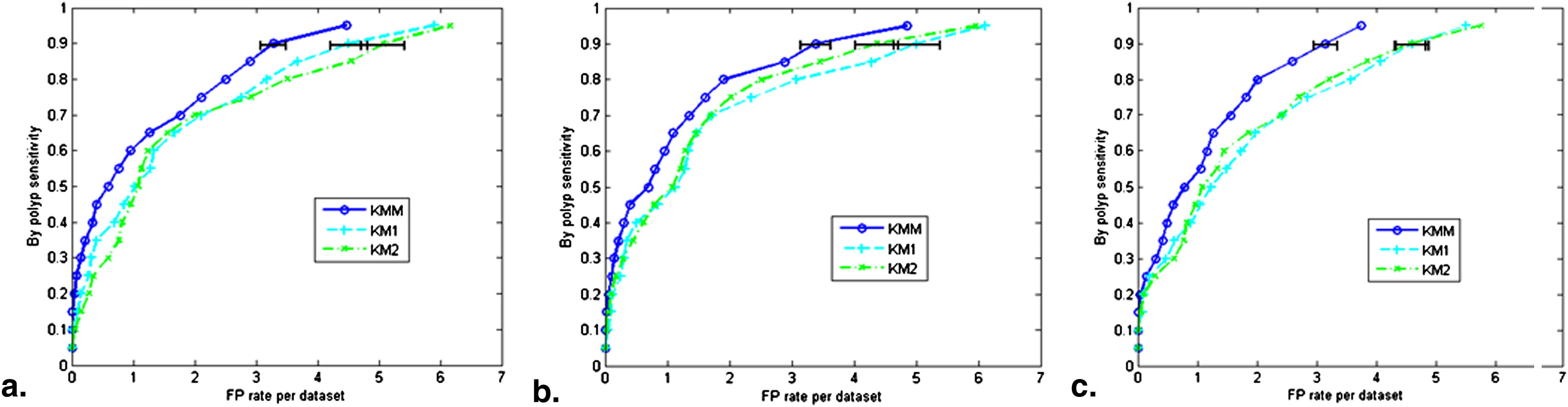
Table 7

False-positive Rates at 90% Detection Sensitivity on the Basis of the Input of the True-positive and False-positive Classification Stage

IPCs Features KM 1 KM 2 KM M KM 1 4.51 (4.21–4.81) 5.07 (4.72–5.42) 3.28 (3.07–3.49) KM 2 5.01 (4.64–5.38) 4.37 (4.02–4.72) 3.38 (3.14–3.62) KM M 4.61 (4.34–4.88) 4.57 (4.31–4.83) 3.15 (2.95–3.35)

IPC, initial polyp candidate; KM M , Knutsson mapping kernel method; KM 1 , kernel method 1; KM 2 , kernel method 2.

In each row, the IPC set is from the same curvature estimation method, but the characterizing features are from various methods.

Table 8

P Values of the Operating Points in Figure 5

IPCs Features KM 1 vs KM 2 KM 1 vs KM M KM 2 vs KM M KM 1 0.14 0.00317 0.000211 KM 2 0.21 0.000531 0.00353 KM M 5.87 0.000342 0.000355

IPC, initial polyp candidate; KM M , Knutsson mapping kernel method; KM 1 , kernel method 1; KM 2 , kernel method 2.

Get Radiology Tree app to read full this article<

Get Radiology Tree app to read full this article<

Get Radiology Tree app to read full this article<

Discussion

Phantom Study

Get Radiology Tree app to read full this article<

Get Radiology Tree app to read full this article<

Patient Study

Get Radiology Tree app to read full this article<

Get Radiology Tree app to read full this article<

Get Radiology Tree app to read full this article<

Get Radiology Tree app to read full this article<

Get Radiology Tree app to read full this article<

Conclusion

Get Radiology Tree app to read full this article<

Get Radiology Tree app to read full this article<

Get Radiology Tree app to read full this article<

Get Radiology Tree app to read full this article<

Get Radiology Tree app to read full this article<

Acknowledgment

Get Radiology Tree app to read full this article<

Get Radiology Tree app to read full this article<

Get Radiology Tree app to read full this article<

References

• 1. American Cancer Society: Cancer facts & figures 2008.2008.American Cancer SocietyAtlanta, GA

• 2. Eddy D.: Screening for colorectal cancer. Ann Intern Med 1990; 113: pp. 373-384.

• 3. Gluecker T., Johnson C., Harmsen W., et. al.: Colorectal cancer screening with CT colonography, colonoscopy, and double-contrast barium enema examination: prospective assessment of patient perceptions and preferences. Radiology 2003; 227: pp. 378-384.

• 4. Levi B., Brooks D., Smith R., et. al.: Emerging technologies in screening for colorectal cancer: CTC, immunochemical fecal occult blood tests, stool screening using molecular markers. CA Cancer J Clin 2002; 53: pp. 44-55.

• 5. Pickhardt P., Choi J., Hwang I., et. al.: Computed tomographic virtual colonoscopy to screen for colorectal neoplasia in asymptomatic adults. N Engl J Med 2003; 349: pp. 2191-2200.

• 6. Kiss G., Cleynenbreugel J., Thomeer M., et. al.: Computer-aided diagnosis in virtual colonography via combination of surface normal and sphere fitting methods. Eur Radiol 2002; 12: pp. 77-81.

• 7. Summers R., Beaulieu C., Pusanik L., et. al.: Automated polyp detector for CT colonography: feasibility study. Radiology 2000; 216: pp. 284-290.

• 8. Summers R., Yao J., Pickhardt P., et. al.: Computed tomographic virtual colonoscopy computer-aided polyp detection in a screening population. Gastroenterology 2005; 129: pp. 1832-1844.

• 9. Taylor S., Halligan S., Burling D., et. al.: Computer-assisted reader software versus expert reviewers for polyp detection on CT colonography. AJR Am J Roentgenol 2006; 186: pp. 696-702.

• 10. Bielen D., Kiss G.: Computer-aided detection for CT colonography: update 2007. Abdom Imaging 2007; 32: pp. 571-581.

• 11. Yoshida H, Nappi J. CAD in CT colonography: past, present, and future. Presented at: 11th International Conference of MICCAI, Workshop on Computational and Visualization Challenges in the New Era of Virtual Colonoscopy; New York, NY; September 6, 2008.

• 12. Monga O., Ayache N., Sander P.T.: From voxel to intrinsic surface features. Image Vis Comput 1992; 10: pp. 403-417.

• 13. Thirion J.P., Gourdon A.: Computing the differential characteristics of isointensity surfaces. Comput Vis Image Understand 1995; 61: pp. 190-202.

• 14. Yoshida H., Nappi J.: Three-dimensional computer-aided diagnosis scheme for detection of colonic polyps. IEEE Trans Med Imaging 2001; 20: pp. 1261-1274.

• 15. Wang Z., Liang Z., Li L., et. al.: Reduction of false positives by internal features for polyp detection in CT-based virtual colonoscopy. Med Phys 2005; 32: pp. 3602-3616.

• 16. Konukoglu E., Acar B., Paik D., et. al.: Polyp enhancing level set evolution of colon wall: method and pilot study. IEEE Trans Med Imaging 2007; 26: pp. 1649-1656.

• 17. van Wijk C., van Ravesteijn V.F., Vos F.M., et. al.: Detection and segmentation of colonic polyps on implicit isosurfaces by second principal curvature flow. IEEE Trans Med Imaging 2010; 29: pp. 688-698.

• 18. Wang S., Zhu H., Lu H., et. al.: Volume-based feature analysis of mucosa for automatic initial polyp detection in virtual colonoscopy. Int J Comput Assist Radiol Surg 2008; 3: pp. 131-142.

• 19. Zhu H., Duan C., Pickhardt P., et. al.: Computer-aided detection of colonic polyps with level set-based adaptive convolution in volumetric mucosa to advance CT colonography toward a screening modality. Cancer Manage Res 2009; 1: pp. 1-13.

• 20. Zhu H., Fan Y., Lu H., et. al.: Improving initial polyp candidate extraction for CT colonography. Phys Med Biol 2010; 55: pp. 2087-2102.

• 21. Zhu H., Liang Z., Pickhardt P., et. al.: Increasing computer-aided detection specificity by projection features for CT colonography. Med Phys 2010; 37: pp. 1468-1481.

• 22. Campbell S., Summers R.: Analysis of kernel method for surface curvature estimation. Int Congr Ser 2004; 1268: pp. 999-1003.

• 23. Rieger R., Timmermans F.J., van Vliet L.J., et. al.: On curvature estimation of ISO surfaces in 3D gray-value images and the computation of shape descriptors. IEEE Trans Patt Anal Mach Intell 2004; 26: pp. 1088-1094.

• 24. Lipschutz M.: Differential geometry.1969.McGraw-HillNew York

• 25. Rieger B, van Vliet LJ. Representing orientation in N-dimensional spaces. In: Petkov N, Westenberg MA, eds. Proceedings of the 10th International Conference on Computer Analysis of Images and Patterns, 2003.

• 26. Knutsson H.: Representing local structures using tensors. Proc Sixth Scand Conf Image Anal 1989; pp. 244-251.

• 27. Liang Z., Wang S.: An EM approach to MAP solution of segmenting tissue mixtures: a numerical analysis. IEEE Trans Med Imaging 2009; 28: pp. 297-310.

• 28. Wang S., Li L., Cohen H., et. al.: An EM approach to MAP solution of segmenting tissue mixture percentages with application to CT-based virtual colonoscopy. Med Phys 2008; 35: pp. 5787-5798.

• 29. Lei T., Sewchand W.: Statistical approach to x-ray CT imaging and its applications in image analysis—part I: statistical analysis of x-ray CT imaging. IEEE Trans Med Imaging 1992; 11: pp. 53-61.

• 30. Chakraboty D., Berbaum K.: Observer studies involving detection and localization: modeling, analysis, and validation. Med Phys 2004; 31: pp. 2313-2330.

• 31. Sundaram P., Zomorodian A., Beauleu C., et. al.: Colon polyp detection using smoothed shape operator: preliminary results. Med Image Anal 2008; 12: pp. 99-119.