Improved Hardware for Higher Spatial Resolution Strain-encoded (SENC) Breast MRI for Strain Measurements

Rationale and Objectives

Early detection of breast lesions using mammography has resulted in lower mortality rates. However, some breast lesions are mammography occult, and magnetic resonance imaging (MRI) is recommended, but it has lower specificity. It is possible to achieve higher specificity by using strain-encoded (SENC) MRI and/or magnetic resonance elastography. SENC breast MRI can measure the strain properties of breast tissue. Similarly, magnetic resonance elastography is used to measure the elasticity (ie, shear stiffness) of different tissue compositions interrogating the tissue mechanical properties. Reports have shown that malignant tumors are three to 13 times stiffer than normal tissue and benign tumors.

Materials and Methods

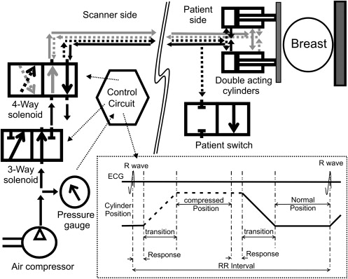
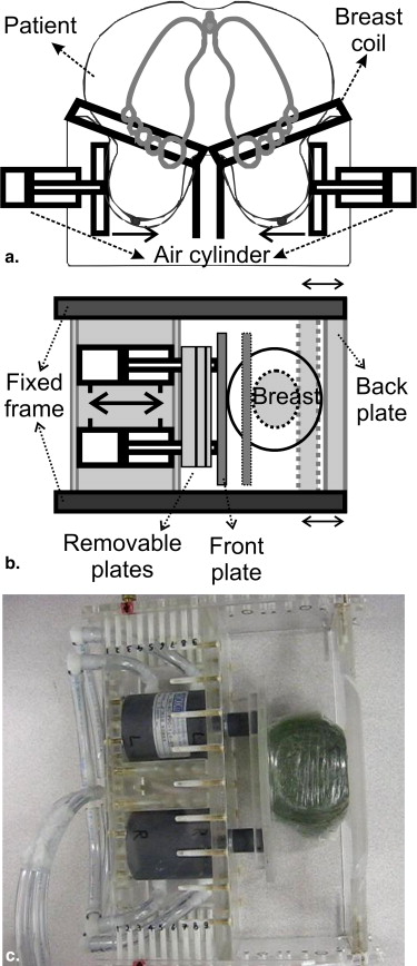
The investigators have developed a SENC breast hardware device capable of periodically compressing the breast, thus allowing for longer scanning time and measuring the strain characteristics of breast tissue. This hardware enables the use of SENC MRI with high spatial resolution (1 × 1 × 5 mm 3 ) instead of fast SENC imaging. Simple controls and multiple safety measures were added to ensure accurate, repeatable, and safe in vivo experiments.

Results

Phantom experiments showed that SENC breast MRI has higher signal-to-noise ratio and contrast-to-noise ratio than fast SENC imaging under different scanning resolutions. Finally, the SENC breast device reproducibility measurements resulted in a difference of <1 mm with a 1% strain difference.

Conclusions

SENC breast magnetic resonance images have higher signal-to-noise ratio and contrast-to-noise ratios than fast SENC images. Thus, combining SENC breast strain measurements with diagnostic breast MRI to differentiate benign from malignant lesions could potentially increase the specificity of diagnosis in the clinical setting.

According to the American Cancer Society’s 2009 report, one in eight women will develop breast cancer in her lifetime. Early detection through periodic screening is the key to lower mortality rates, and the current methods used are mammography and ultrasound. However, some breast lesions are mammography and ultrasound occult (ie, those in dense breasts). Therefore, other methods, such as magnetic resonance imaging (MRI), are used especially in women who are at high risk to develop breast cancer.

Although MRI has high sensitivity (95%), its specificity remains moderate (83%) , and there is a need to increase specificity so that the number of unnecessary biopsy procedures can be reduced. Recent MRI methods have been proposed to further improve specificity, including diffusion-weighted imaging and apparent diffusion coefficient (DWI/ADC) mapping , magnetic resonance spectroscopy , and magnetic resonance elastography (MRE) , all of which were reviewed by El Khouli et al . DWI/ADC mapping can probe the movement of water and provide a measure of cellularity. Magnetic resonance spectroscopy can give metabolic information on the breast tissue.

Get Radiology Tree app to read full this article<

Methods

Hardware

Get Radiology Tree app to read full this article<

SENC breast hardware on the scanner side

Get Radiology Tree app to read full this article<

SENC breast hardware on the patient side

Get Radiology Tree app to read full this article<

SENC breast hardware modes of operation

Get Radiology Tree app to read full this article<

SENC MRI

Get Radiology Tree app to read full this article<

ϵ=ΔLL0=L−L0L0=LL0−1, ϵ

−

where Δ L is the change of the tissue’s length, and L and L 0 are the final and initial lengths of the tissue, respectively.

Get Radiology Tree app to read full this article<

ω(p)=ωLIL(p)+ωHIH(p)IL(p)+IH(p), ω

(

)

(

)

(

)

(

)

(

)

and local strain can then be quantified as

ϵ(p)=ω0ω(p)−1. ϵ

(

)

(

)

−

Get Radiology Tree app to read full this article<

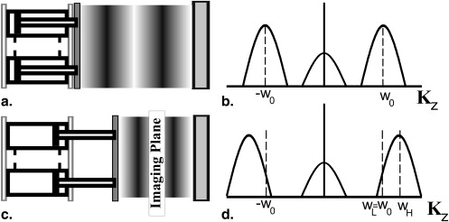
Tagging Frequency

Get Radiology Tree app to read full this article<

ωH=ω0ϵmax stretch+1+B,ωL=ω0ϵmax compression+1−B,ω0=B(ϵmax compression+1)(ϵmax stretch+1)(ϵmax stretch−ϵmax compression), ω

max stretch

max compression

−

(

max compression

)

(

max stretch

)

(

max stretch

−

max compression

)

where B = (1/slice thickness), and ϵ max compression and ϵ max stretch are the expected strain values externally applied by our device. Note that ϵ max compression is always expressed in negative values, while ϵ max stretch is expressed in positive values. Because we are only interested in compression, we set ϵ max stretch to zero. Therefore, equation 3 is simplified to

ωL=ω0=−Bϵmax compression−B,ωH=ωL+B. ω

−

max compression

−

Get Radiology Tree app to read full this article<

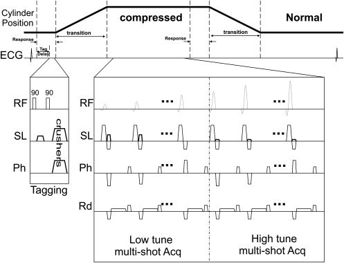
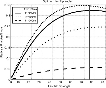
Pulse Sequence and Flip Angle Optimization

Get Radiology Tree app to read full this article<

Ik∝MSSTAG(z)exp(−Δt/T1)∏k−1j=1cos(αj)sin(αk), I

∝

TAG

(

)

exp

(

−

)

∏

−

cos

(

)

sin

(

)

where M SS is the steady state magnetization, TAG( z ) is the tagging pattern created in the slice selection direction, Δ t is the time between each radiofrequency (RF) pulse, T1 is the relaxation time of the tissue, and α j is the flip angle of the j th RF pulse. To compensate for this signal loss, Stuber et al proposed increasing the excitation flip angle, α j , gradually through time to maintain uniform signal intensity through time using

αk−1=atan[sin(αk)exp(−Δt/T1)]. α

−

atan

[

sin

(

)

exp

(

−Δ

)

]

Get Radiology Tree app to read full this article<

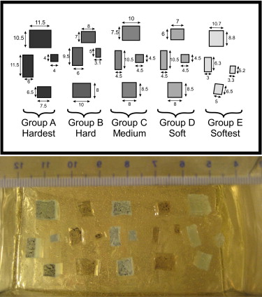
Phantom design and experiments

Phantom Composition

Get Radiology Tree app to read full this article<

Table 1

Mixing Ratio for Different Masses with Corresponding Young’s Modulus Measured Using Dynamic Mechanical Analyzer

Group Material Mixing Ratio Young’s Modulus (KPa) Group/Background Ratio Classification A 3-4207 Dielectric Tough Gel ∗ 1:1 593 8.4 Malignant B 3-4133 Dielectric Gel ∗ 1.5:1 226 3.2 Benign C 3-4207 Dielectric Tough Gel ∗ 1:1.2 171 2.4 Benign D 3-4133 Dielectric Gel ∗ 1.2:1 100 1.4 Normal Background A-341 gel † 1:10 71 1 Normal E 3-4222 Dielectric Firm Gel ∗ 1:1.5 11–20 0.15–0.3 Normal

Get Radiology Tree app to read full this article<

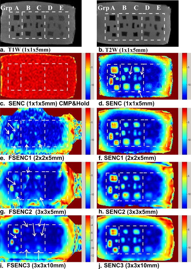
MRI Scanning Protocol

Get Radiology Tree app to read full this article<

Table 2

Scanning Parameters for T1W, T2W, and Different Variations of SENC and FSENC Scans

Scan In-plane Resolution (mm) Slice Thickness (mm) ω_L = ω_0 (mm −1 ) ω H (mm −1 ) TFE Factor TSE Factor EPI Factor Compression Cycle/Slice Total Scan time (seconds) for Five Slices T1W 1 × 1 5 — — 3 — — 39 T2W 1 × 1 5 — — 12 — — 67 SENC 1 × 1 5 1.132 1.332 10 None 19 190 SENC1 2 × 2 5 1.132 1.332 10 None 9 90 SENC2 3 × 3 5 1.132 1.332 10 None 6 60 SENC3 3 × 3 10 0.567 0.667 10 None 6 60 FSENC1 2 × 2 5 1.132 1.332 17 3 1 10 FSENC2 3 × 3 5 1.132 1.332 11 3 1 10 FSENC3 3 × 3 10 0.567 0.667 11 3 1 10

EPI, echo-planar imaging; FSENC, fast strain-encoded; SENC, strain-encoded; TFE, turbo field-echo; T1W, T1-weighted; TSE, turbo spin-echo; T2W, T2-weighted.

T1W and T2W images are scanned while the device is in compress-and-hold mode.

Get Radiology Tree app to read full this article<

Quantification

Get Radiology Tree app to read full this article<

SNR=Sbackgroundσnoise, SNR

background

noise

where S is the mean signal intensity in the phantom background, and σ is the standard deviation of the noise calculated from a 30 × 30 pixel rectangular area outside the phantom. Because we were interested in detecting and measuring tumor size, we used the CNR elastography (CNR e ) given by Bilgen :

CNRe=2(Stumor−Sbackground)2σ2tumor+σ2background, CNR

(

tumor

−

background

)

tumor

background

where the background was calculated by including the pixels inside a circle surrounding the masses and then excluding pixels inside the masses.

Get Radiology Tree app to read full this article<

SENC Breast Hardware Accuracy

Get Radiology Tree app to read full this article<

Results

Get Radiology Tree app to read full this article<

Table 3

SNR and CNR e of Different Mass Groups for T1W, T2W, SENC, and FSENC Scans

Scan SNR CNR e Group A Group B Group C Group D Group E T1W 750 ± 20 19 ± 11 37 ± 22 49 ± 23 40 ± 22 21 ± 6 T2W 880 ± 10 35 ± 11 34 ± 32 50 ± 19 41 ± 28 23 ± 16 SENC 45 ± 5 80 ± 31 47 ± 18 40 ± 6 — — SENC1 60 ± 5 50 ± 29 33 ± 17 27 ± 10 — — SENC2 65 ± 9 38 ± 24 28 ± 10 25 ± 5 — — SENC3 150 ± 15 29 ± 19 31 ± 17 24 ± 5 — — FSENC1 22 ± 3 7.8 ± 5.5 2.2 ± 2.2 2.7 ± 3 — — FSENC2 54 ± 4 9.1 ± 5.6 1.8 ± 0.9 4.3 ± 3 — — FSENC3 110 ± 10 10 ± 7 1 ± 2 5 ± 7 — —

CNRe, contrast-to-noise ratio elastography; FSENC, fast strain-encoded; SENC, strain-encoded; SNR, signal-to-noise ratio; T1W, T1-weighted; T2W, T2-weighted.

Get Radiology Tree app to read full this article<

Discussion

Get Radiology Tree app to read full this article<

Conclusion

Get Radiology Tree app to read full this article<

References

1. American Cancer Society. Cancer facts & figures 2009. Available at: http://www.cancer.org/acs/groups/content/@nho/documents/document/500809webpdf.pdf . Accessed February 11, 2011.
2. Bluemke D.A., Gatsonis C., Chen M., et. al.: Magnetic resonance imaging of the breast prior to biopsy. JAMA 2004; 292: pp. 2735-2742.
3. Lehman C., Gatsonis C., Kuhl C., et. al.: MRI evaluation of the contralateral breast in women with recently diagnosed breast cancer. N Engl J Med 2007; 356: pp. 1295-1303.
4. Kuroki Y., Nasu K., Kuroki S., et. al.: Diffusion-weighted imaging of breast cancer with the sensitivity encoding technique: analysis of the apparent diffusion coefficient value. Magn Reson Med Sci 2004; 3: pp. 79-85.
5. Jin G., An N., Jacobs M.A., et. al.: The role of parallel diffusion-weighted imaging and apparent diffusion coefficient (ADC) map values for evaluating breast lesions: preliminary results. Acad Radiol 2010; 17: pp. 456-463.
6. Guo Y., Cai Y., Cai Z., et. al.: Differentiation of clinically benign and malignant breast lesions using diffusion-weighted imaging. J Magn Reson Imaging 2002; 16: pp. 172-178.
7. El Khouli R.H., Jacobs M.A., Mezban S.D., et. al.: Diffusion-weighted imaging improves the diagnostic accuracy of conventional 3.0-T breast MR imaging. Radiology 2010; 256: pp. 64-73.
8. Kvistad K., Bakken I., Gribbestad I., et. al.: Characterization of neoplastic and normal human breast tissues with in vivo 1H MR spectroscopy. J Magn Reson Imaging 1999; 10: pp. 159-164.
9. Yeung D., Cheung H., Tse G.: Human breast lesions: characterization with contrast-enhanced in vivo proton MR spectroscopy: initial results. Radiology 2001; 220: pp. 40-46.
10. Roebuck J., Cecil K., Schnall M., et. al.: Human breast lesions: characterization with proton MR spectroscopy. Radiology 1998; 209: pp. 269-275.
11. Katz-Brull R., Lavin P., Lenkinski R.: Clinical utility of proton magnetic resonance spectroscopy in characterizing breast lesions. J Natl Cancer Inst 2002; 94: pp. 1197-1203.
12. Jacobs M.A., Barker P., Bottomley P., et. al.: Proton magnetic resonance spectroscopic imaging of human breast cancer: a preliminary study. J Magn Reson Imaging 2004; 19: pp. 68-75.
13. Manduca A., Oliphant T., Dresner M., et. al.: Magnetic resonance elastography: non-invasive mapping of tissue elasticity. Med Image Anal 2001; 5: pp. 237-254.
14. Sinkus R., Lorenzen J., Schrader D., et. al.: High-resolution tensor MR elastography for breast tumour detection. Phys Med Biol 2000; 45: pp. 1649-1664.
15. Sinkus R., Tanter M., Catheline S., et. al.: Imaging anisotropic and viscous properties of breast tissue by magnetic resonance-elastography. Magn Reson Med 2005; 53: pp. 372-387.
16. El Khouli R.H., Jacobs M.A., Bluemke D.A.: Magnetic resonance imaging of the breast. Semin Roentgenol 2008; 43: pp. 265-281.
17. Sinkus R., Siegmann K., Xydeas T., et. al.: MR elastography of breast lesions: understanding the solid/liquid duality can improve the specificity of contrast-enhanced MR mammography. Magn Reson Med 2007; 58: pp. 1135-1144.
18. Asbach P., Klatt D., Hamhaber U., et. al.: Assessment of liver viscoelasticity using multifrequency MR elastography. Magn Reson Med 2008; 60: pp. 373-379.
19. Huwart L., Peeters F., Sinkus R., et. al.: Liver fibrosis: non-invasive assessment with MR elastography. NMR Biomed 2006; 19: pp. 173-179.
20. Huwart L., Sempoux C., Vicaut E., et. al.: Magnetic resonance elastography for the noninvasive staging of liver fibrosis. Gastroenterology 2008; 135: pp. 32-40.
21. Kruse S., Rose G., Glaser K., et. al.: Magnetic resonance elastography of the brain. Neuroimage 2008; 39: pp. 231-237.
22. Sack I., Beierbach B., Hamhaber U., et. al.: Non-invasive measurement of brain viscoelasticity using magnetic resonance elastography. NMR Biomed 2008; 21: pp. 265-271.
23. Kemper J., Sinkus R., Lorenzen J., et. al.: MR elastography of the prostate: initial in-vivo application. Rofo 2004; 176: pp. 1094-1099.
24. Sack I., Rump J., Elgeti T., et. al.: MR elastography of the human heart: noninvasive assessment of myocardial elasticity changes by shear wave amplitude variations. Magn Reson Med 2008; 61: pp. 668-677.
25. Uffmann K., Maderwald S., Ajaj W., et. al.: In vivo elasticity measurements of extremity skeletal muscle with MR elastography. NMR Biomed 2004; 17: pp. 181-190.
26. Papazoglou S., Rump J., Braun J., et. al.: Shear wave group velocity inversion in MR elastography of human skeletal muscle. Magn Reson Med 2006; 56: pp. 489-497.
27. Tse Z., Janssen H., Hamed A., et. al.: Magnetic resonance elastography hardware design: a survey. J Eng Med 2009; 223: pp. 497-514.
28. O’Donnell M.: NMR blood flow imaging using multiecho, phase contrast sequences. Med Phys 1985; 12: pp. 59-64.
29. Pelc N., Herfkens R., Shimakawa A., et. al.: Phase contrast cine magnetic resonance imaging. Magn Reson Q 1991; 7: pp. 229-254.
30. Bernstein M., Ikezaki Y.: Comparison of phase-difference and complex-difference processing in phase-contrast MR angiography. J Magn Reson Imaging 2005; 1: pp. 725-729.
31. Plewes D., Bishop J., Samani A., et. al.: Visualization and quantification of breast cancer biomechanical properties with magnetic resonance elastography. Phys Med Biol 2000; 45: pp. 1591-1610.
32. Rossman P., Muthupillai R., Ehman R.: Driver device for MR elastography. US Patent No 5,952,828 September, 14 1999;
33. Doyley M., Weaver J., Van Houten E., et. al.: Thresholds for detecting and characterizing focal lesions using steady state MR elastography. Med Phys 2003; 30: pp. 495-504.
34. Osman N., Sampath S., Atalar E., et. al.: Imaging longitudinal cardiac strain on short-axis images using strain-encoded MRI. Magn Reson Med 2001; 46: pp. 324-334.
35. Osman N.: Detecting stiff masses using strain-encoded (SENC) imaging. Magn Reson Med 2003; 49: pp. 606-608.
36. Pan L., Stuber M., Kraitchman D., et. al.: Real-time imaging of regional myocardial function using fast-SENC. Magn Reson Med 2006; 55: pp. 386-395.
37. Fahmy A., Krieger A., Osman N.: An integrated system for real-time detection of stiff masses with a single compression. IEEE Trans Biomed Eng 2006; 53: pp. 1286-1293.
38. Yousef T., Osman N.: Effect of noise and slice profile on strain quantifications of strain encoding (SENC) MRI. Lect Notes Comput Sci 2007; 4466: pp. 50-59.
39. Fischer S., McKinnon G., Maier S., et. al.: Improved myocardial tagging contrast. Magn Reson Med 1993; 30: pp. 191-200.
40. Stuber M., Spiegel M., Fischer S., et. al.: Single breath-hold slice-following CSPAMM myocardial tagging. Magn Reson Mat Phys Biol Med 1999; 9: pp. 85-91.
41. Samani A., Zubovits J., Plewes D.: Elastic moduli of normal and pathological human breast tissues: an inversion-technique-based investigation of 169 samples. Phys Med Biol 2007; 52: pp. 1565-1576.
42. Bilgen M.: Target detectability in acoustic elastography. IEEE Trans Ultrason Ferroelectr Freq Contr 1999; 46: pp. 1128-1133.

Improved Hardware for Higher Spatial Resolution Strain-encoded (SENC) Breast MRI for Strain Measurements

Rationale and Objectives

Materials and Methods

Results

Conclusions

Methods

Hardware

SENC breast hardware on the scanner side

SENC breast hardware on the patient side

SENC breast hardware modes of operation

SENC MRI

Tagging Frequency

Pulse Sequence and Flip Angle Optimization

Phantom design and experiments

Phantom Composition

MRI Scanning Protocol

Quantification

SENC Breast Hardware Accuracy

Results

Discussion

Conclusion

References

Further Reading

Accurate Prostate Volume Estimation Using Multifeature Active Shape Models on T2-weighted MRI

Assessment of Left Ventricular Function and Mass by MR Imaging

Brain and Spine Imaging Patterns