
Rationale and Objectives
To evaluate the improvements in measurements of blood flow (BF), blood volume (BV), and permeability–surface area product (PS) after principal component analysis (PCA) filtering of computed tomography (CT) perfusion images. To evaluate the improvement in CT perfusion image quality with poor contrast-to-noise ratio (CNR) in vivo.
Materials and Methods
A digital phantom with CT perfusion images reflecting known values of BF, BV, and PS was created and was filtered using PCA. Intraclass correlation coefficients and Bland–Altman analysis were used to assess reliability of measurements and reduction in measurement errors, respectively. Rats with C6 gliomas were imaged using CT perfusion, and the raw CT perfusion images were filtered using PCA. Differences in CNR, BF, BV, and PS before and after PCA filtering were assessed using repeated measures analysis of variance.
Results
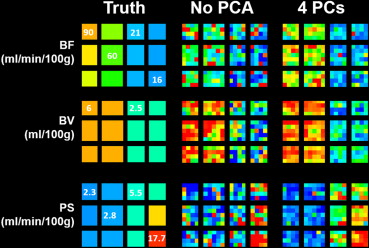
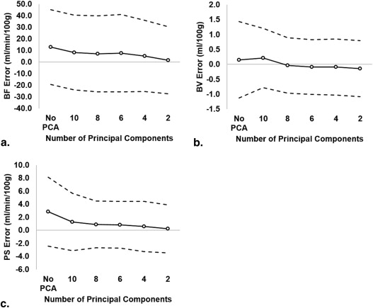
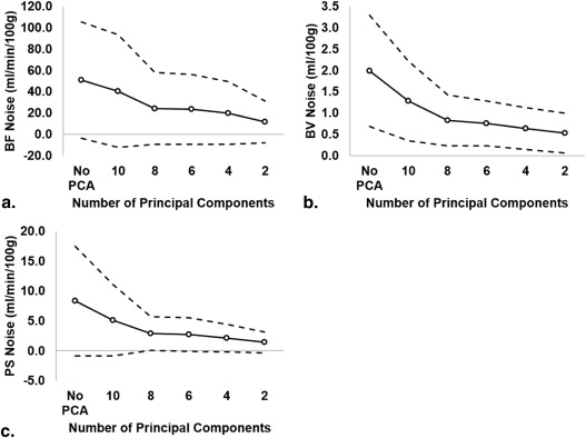
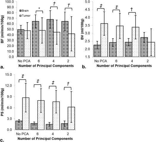
From simulation, mean errors decreased from 12.8 (95% confidence interval [CI] = −19.5 to 45.0) to 1.4 mL/min/100 g (CI = −27.6 to 30.4), 0.2 (CI = −1.1 to 1.4) to −0.1 mL/100 g (CI = −1.1 to 0.8), and 2.9 (CI = −2.4 to 8.1) to 0.2 mL/min/100 g (CI = −3.5 to 3.9) for BF, BV, and PS, respectively. Map noise in BF, BV, and PS were decreased from 51.0 (CI = −3.5 to 105.5) to 11.6 mL/min/100 g (CI = −7.9 to 31.2), 2.0 (CI = 0.7 to 3.3) to 0.5 mL/100 g (CI = 0.1 to 1.0), and 8.3 (CI = −0.8 to 17.5) to 1.4 mL/min/100 g (CI = −0.4 to 3.1), respectively. For experiments, CNR significantly improved with PCA filtering in normal brain ( P < .05) and tumor ( P < .05). Tumor and brain BFs were significantly different from each other after PCA filtering with four principal components ( P < .05).
Conclusions
PCA improved image CNR in vivo and reduced the measurement errors of BF, BV, and PS from simulation. A minimum of four principal components is recommended.
Computed tomography (CT) perfusion is a diagnostic tool for the evaluation of acute ischemic stroke, and it is becoming increasingly used for measuring blood flow (BF), blood volume (BV), and permeability–surface area product (PS) in malignant brain tumors . The measurements of BF, BV, and PS in tumors are affected by CT perfusion image contrast-to-noise ratio (CNR). Recently, Balvay et al. showed that filtering CT perfusion images with principal component analysis (PCA) improved CNR in CT perfusion images of patients with ovarian and metastatic renal tumors. It is not known whether PCA can improve CNR of CT perfusion images of patients with malignant brain tumors, which have a lower CNR because of lower tumor blood flow in the brain compared to other malignancies such as metastatic renal tumors . In preclinical imaging of cancer models with a clinical CT scanner, a high spatial resolution is desirable to detect small tumors. However, CNR from scanning small animals is low because: (1) image noise increases with higher spatial resolution (ie, smaller pixel size); and (2) the effect of partial volume averaging is more prominent in small animals than in humans. Therefore, we hypothesized that CT perfusion images of a preclinical model of malignant glioma are useful to evaluate the ability of PCA in improving image quality under low-CNR condition. It has not been demonstrated that an increase in CNR after PCA filtering improves the measurements of BF, BV, and PS. Accurate and precise measurements of these parameters are important because they have been shown to be valuable for grading gliomas and for distinguishing recurrent tumor from treatment-induced necrosis .
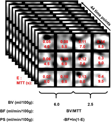
In this study, we first designed a digital phantom to validate PCA image filtering by comparing the accuracies and precisions of BF, BV, and PS without and with PCA filtering of simulated CT perfusion images. We then evaluated the improvement in CNR and changes in BF, BV, and PS measurements after PCA filtering CT perfusion images of a malignant rat glioma model.
Materials and methods
Validation of PCA by Simulation
Get Radiology Tree app to read full this article<
Get Radiology Tree app to read full this article<
Get Radiology Tree app to read full this article<
Principal Component Analysis
Get Radiology Tree app to read full this article<
In vivo Experiments
Get Radiology Tree app to read full this article<
Assessment of Image Quality and Information Loss after PCA Filtering
Get Radiology Tree app to read full this article<
Get Radiology Tree app to read full this article<
Get Radiology Tree app to read full this article<
Calculation of BF, BV, and PS
Get Radiology Tree app to read full this article<
Statistical Analysis
Get Radiology Tree app to read full this article<
Get Radiology Tree app to read full this article<
Results
Get Radiology Tree app to read full this article<
Table 1
Intraclass Correlation of Different Computed Tomography Perfusion Parameters with the True Values
Number of PCs BF BV PS Intraclass Correlation Coefficient (95% CI)P Value ∗ Intraclass Correlation Coefficient (95% CI)P Value † Intraclass Correlation Coefficient (95% CI)P Value ‡ No PCA 0.73 (0.34–0.86) .57 0.96 (0.95–0.97) .42 0.77 (0.16–0.91) .59 Ten PCs 0.79 (0.64–0.87) .19 0.98 (0.96–0.98) .05 0.87 (0.73–0.93) .06 Eight PCs 0.79 (0.68–0.86) .12 0.98 (0.97–0.99) .00 § 0.91 (0.83–0.95) .00 § Six PCs 0.79 (0.66–0.86) .15 0.98 (0.97–0.99) .00 § 0.91 (0.84–0.94) .00 § Four PCs 0.82 (0.75–0.87) .01 § 0.98 (0.97–0.98) .00 § 0.90 (0.87–0.93) .00 § Two PCs 0.82 (0.77–0.86) .00 § 0.98 (0.97–0.98) .00 § 0.92 (0.89–0.94) .00 §
BF, blood flow; BV, blood volume; CI, confidence interval; PCs, principal components; PCA, principal component analysis; PS, permeability–surface area product.
Get Radiology Tree app to read full this article<
Get Radiology Tree app to read full this article<
Get Radiology Tree app to read full this article<
Get Radiology Tree app to read full this article<
Get Radiology Tree app to read full this article<
Get Radiology Tree app to read full this article<
Table 2
Evaluation of Quality of Computed Tomography Perfusion Images Filtering
Number of PCs Noise Level ± SD (HU) CNR ± SD Percentage of Voxels with FRI ≥ 5% Brain Tumor Brain Tumor Brain Tumor No PCA 16.9 ± 0.5 16.6 ± 0.6 0.6 ± 0.1 1.4 ± 0.4 NA NA Six PCs 5.2 ± 0.6 ∗ 5.6 ± 0.6 ∗ 1.9 ± 0.3 ∗ 3.8 ± 1.2 ∗ 0.2 ± 0.2 0.3 ± 0.5 Four PCs 3.3 ± 0.4 ∗ 3.9 ± 0.7 ∗ 2.9 ± 0.4 ∗ 5.5 ± 2.4 ∗ 0.5 ± 0.3 1.1 ± 1.0 Two PCs 1.6 ± 0.3 ∗ 2.2 ± 0.6 ∗ 6.2 ± 1.3 ∗ 6.5 ± 1.8 ∗ 4.2 ± 2.2 26.4 ± 14.2
CNR, contrast-to-noise ratio; FRI, fractional residual information; HU, Hounsfield unit; NA, not applicable; PCs, principal components; PCA, principal component analysis; SD, standard deviation.
Get Radiology Tree app to read full this article<
Table 3
P Values of Repeated Measures Analysis of Variance for Measurements of BF, BV, and PS
Factor BF BV PS PCA 0.21 <0.02 <0.01 Region <0.05 <0.03 <0.01 Interaction between PCA and region <0.01 <0.01 <0.01
BF, blood flow; BV, blood volume; PCA, principal component analysis; PS, permeability–surface area product.
Get Radiology Tree app to read full this article<
Discussion
Get Radiology Tree app to read full this article<
Get Radiology Tree app to read full this article<
Get Radiology Tree app to read full this article<
Get Radiology Tree app to read full this article<
Get Radiology Tree app to read full this article<
Conclusions
Get Radiology Tree app to read full this article<
Appendix 1
Simulation of time-attenuation curves
Get Radiology Tree app to read full this article<
Q(t)=BF⋅Ca(t)⊗H(t)=Ca(t)⊗[BF⋅H(t)] Q
(
t
)
=
BF
⋅
C
a
(
t
)
⊗
H
(
t
)
=
C
a
(
t
)
⊗
[
BF
⋅
H
(
t
)
]
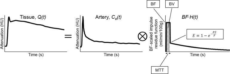
where BF is blood flow, C__a__(t) is the arterial TAC (also known as the arterial input function), ⊗ ⊗ is the convolution operator, H(t) is the impulse residue function. This mathematical operation is graphically illustrated in Supplementary Figure 1 . The arterial TAC used in this simulation was a population-averaged arterial TAC. The impulse residue function describes the fraction of contrast that remains in the tissue as a function of time after a bolus injection into the arterial inlet. The blood flow–scaled impulse residue function, BF⋅H(t) B
F
⋅
H
(
t
) , has two phases. The first phase is a rectangular function with a height of BF that is maintained for the duration of the mean transit time and has an area equal to blood volume (BV). It represents the retention of contrast in the tissue region before venous outflow. The second phase starts at a height of the extraction fraction and decays exponentially; it describes back flux of extravasated contrast from the interstitial space into the intravascular space.
Get Radiology Tree app to read full this article<
Appendix 2
Principal component analysis filtering of CT perfusion images
Get Radiology Tree app to read full this article<
Q˜p=∑Ni=1wip⋅ai Q
˜
p
=
∑
i
=
1
N
w
i
p
·
a
i
where N is the number of principal components with the largest variances used to noise filter Qp Q
p , a__i is the i th Eigen vector and w__ip is the corresponding weight which can be calculated as:
wip=aTi⋅(Qp−Q¯¯¯) w
i
p
=
a
i
T
·
(
Q
p
−
Q
¯
)
where Q¯¯¯ Q
¯ is the mean of all TACs and aTi a
i
T is the transpose of a__i .
Get Radiology Tree app to read full this article<
Appendix 3
Fractional residual information
Get Radiology Tree app to read full this article<
FRIp=∥Sp∥2∥Rp∥2=∥Sp∥2∥Sp+Np∥2 FRI
p
=
‖
S
p
‖
2
‖
R
p
‖
2
=
‖
S
p
‖
2
‖
S
p
+
N
p
‖
2
Get Radiology Tree app to read full this article<
Get Radiology Tree app to read full this article<
Cp(k)=1m−|k|∑m−ki=1Rp(i)⋅Rp(i+k) C
p
(
k
)
=
1
m
−
|
k
|
∑
i
=
1
m
−
k
R
p
(
i
)
·
R
p
(
i
+
k
)
where m is the number of time points, k is the time lag and R__p__(i) is the i th element of the m × 1 residual vector R__p . C__p__(k) can identify signal ( S__p ) hidden in the noise ( N__p ) of R__p in the following way. In general, the autocorrelations of N__p and S__p are approximately zero for time lag k > k__n and k__s , respectively. If k__s > k__n , then the autocorrelation of the residual C__p__(k) can be used to approximate S__p for time lag k__n < k < k__s . In particular, extrapolation of C__p__(k) in the range k__n < k < k__s to k = 0 will give the autocorrelation of S__p at k = 0, which by analogy to Equation 2 gives ∥Sp∥2 ‖
S
p
‖
2 when multiplied by ( m−|k| ). We used a second-order polynomial to extrapolate C__p__(k) in the range k__n < k < k__s to k = 0. The k__n and k__s used were fixed to 1 and 30 time lags, respectively.
Get Radiology Tree app to read full this article<
Supplementary Data
Get Radiology Tree app to read full this article<
Get Radiology Tree app to read full this article<
Get Radiology Tree app to read full this article<
References
1. Jain R.: Perfusion CT imaging of brain tumors: an overview. AJNR Am J Neuroradiol 2011; 32: pp. 1570-1577.
2. Balvay D., Kachenoura N., Espinoza S., et. al.: Signal-to-noise ratio improvement in dynamic contrast-enhanced CT and MR imaging with automated principal component analysis filtering. Radiology 2011; 258: pp. 435-445.
3. Fournier L.S., Oudard S., Thiam R., et. al.: Metastatic renal carcinoma: evaluation of antiangiogenic therapy with dynamic contrast-enhanced CT. Radiology 2010; 256: pp. 511-518.
4. Kremer S., Grand S., Berger F., et. al.: Dynamic contrast-enhanced MRI: differentiating melanoma and renal carcinoma metastases from high-grade astrocytomas and other metastases. Neuroradiology 2003; 45: pp. 44-49.
5. Bulakbasi N., Kocaoglu M., Farzaliyev A., et. al.: Assessment of diagnostic accuracy of perfusion MR imaging in primary and metastatic solitary malignant brain tumors. AJNR Am J Neuroradiol 2005; 26: pp. 2187-2199.
6. Jain R., Ellika S.K., Scarpace L., et. al.: Quantitative estimation of permeability surface-area product in astroglial brain tumors using perfusion CT and correlation with histopathologic grade. AJNR Am J Neuroradiol 2008; 29: pp. 694-700.
7. Jain R., Narang J., Schultz L., et. al.: Permeability estimates in histopathology-proved treatment-induced necrosis using perfusion CT: can these add to other perfusion parameters in differentiating from recurrent/progressive tumors?. AJNR Am J Neuroradiol 2011; 32: pp. 658-663.
8. Lee T.Y., Purdie T.G., Stewart E.: CT imaging of angiogenesis. Q J Nucl Med 2003; 47: pp. 171-187.
9. Johnson J.A., Wilson T.A.: A model for capillary exchange. Am J Physiol 1966; 210: pp. 1299-1303.
10. Paxinos G., Watson C.: The rat brain.Stereotaxic coordinates.2007.Academic PressBurlington:
11. Shrout P.E., Fleiss J.L.: Intraclass correlations: uses in assessing rater reliability. Psychol Bull 1979; 86: pp. 420-428.
12. Bland J.M., Altman D.G.: Statistical methods for assessing agreement between two methods of clinical measurement. Lancet 1986; 1: pp. 307-310.
13. Norušis M.J.: SPSS ® Statistics 17.0: statistical procedure companion.2008.Prentice Hall IncUpper Saddle River, NJpp. 599-609.
14. Zhang K., Sejnowski T.J.: A universal scaling law between gray matter and white matter of cerebral cortex. Proc Natl Acad Sci U S A 2000; 97: pp. 5621-5626.
15. Balvay D., Troprès I., Billet R., et. al.: Mapping the zonal organization of tumor perfusion and permeability in a rat glioma model by using dynamic contrast-enhanced synchrotron radiation CT. Radiology 2009; 250: pp. 692-702.
16. Ren Q., Dewan S.K., Li M., et. al.: Comparison of adaptive statistical iterative and filtered back projection reconstruction techniques in brain CT. Eur J Radiol 2012; 81: pp. 2597-2601.
17. Yeung T.P., Yartsev S., Bauman G., et. al.: The effect of scan duration on the measurement of perfusion parameters in CT perfusion studies of brain tumors. Acad Radiol 2013; 20: pp. 59-65.
18. Cenic A., Nabavi D.G., Craen R.A., et. al.: A CT method to measure hemodynamics in brain tumors: validation and application of cerebral blood flow maps. AJNR Am J Neuroradiol 2000; 21: pp. 462-470.
19. Kudo K., Christensen S., Sasaki M., et. al.: Accuracy and reliability assessment of CT and MR perfusion analysis software using a digital phantom. Radiology 2013; 267: pp. 201-211.