
Rationale and Objectives
The acceptance of computer-assisted diagnosis (CAD) in clinical practice has been constrained by the scarcity of identifiable biologic correlates for CAD-based image parameters. This study aims to identify biologic correlates for computed tomography (CT) liver texture in a series of patients with colorectal cancer.
Materials and Methods
In 28 patients with colorectal cancer, total hepatic perfusion (THP), hepatic arterial perfusion, and hepatic portal perfusion (HPP) were measured using perfusion CT. Hepatic glucose use was also determined from positron emission tomography (PET) and expressed as standardized uptake value (SUV). A hepatic phosphorylation fraction index (HPFI) was determined from both SUV and THP. These physiologic parameters were correlated with CAD parameters namely hepatic densitometry, selective-scale, and relative-scale texture features in apparently normal areas of portal-phase hepatic CT.
Results
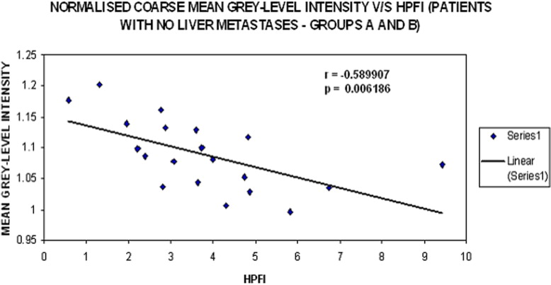
For patients without liver metastases, a relative-scale texture parameter correlated inversely with SUV ( r = −0.587, P = .007) and, positively with THP ( r = 0.512, P = .021) and HPP ( r = 0.451, P = .046). However, this relative texture parameter correlated most significantly with HPFI ( r = −0.590, P = .006). For patients with liver metastases, although not significant an opposite trend was observed between these physiologic parameters and relative texture features (THP: r < −0.4, HPFI: r > 0.35).
Conclusion
Total hepatic blood flow and glucose metabolism are two distinct but related biologic correlates for liver texture on portal phase CT, providing a rationale for the use of hepatic texture analysis as a indicator for patients with colorectal cancer.
Radiologists’ assessment of diagnostic images is largely based on evaluating morphologic information such as size and shape and the human visual system has difficulties in discriminating textural information such as coarseness and regularity that result from local spatial variations in image brightness ( ). Also, image perception and identifying relationships between perceived patterns and possible diagnosis heavily depend on radiologist’s knowledge, memory, intuition, and diligence. The use of texture analysis in computer-aided diagnosis (CAD) of radiologic images has therefore attracted a lot of interest. Texture is a rich source of visual information and a key component in image analysis and understanding in humans ( ), with evidence showing texture mechanisms and discrimination to be beneficial in perceptual learning ( ). Algorithmic processing as against visual analysis is becoming increasingly important for deriving quantitative textural information from images.
Although there seems to be a great potential for texture analysis as a CAD technique in medical imaging, very few of these techniques have actually been put into clinical practice. One of the few commercialized applications of image processing that has withstood thorough testing and gained approval from the US Food and Drug Administration is Image Checker M1000 (R2 Technology, Los Altos, CA) for screening mammograms. One potential reason constraining the acceptance of CAD despite demonstrable improvements in diagnostic performance in many cases may be a paucity of identifiable biologic correlates for the image parameters underlying the CAD. Whereas tissue microcalcification is a likely correlate for mammographic computer analysis, the correlates for other organs may be less clear. The identification of biologic correlates is further impaired when there are difficulties in obtaining tissue for histologic analysis from the invasive nature of biopsy in some organs—for instance, the brain or liver. In these circumstances, physiologic correlates such as those provided by functional imaging techniques may be more appropriate than pathologic features.
Get Radiology Tree app to read full this article<
Get Radiology Tree app to read full this article<
Get Radiology Tree app to read full this article<
Materials and methods
Patients
Get Radiology Tree app to read full this article<
Get Radiology Tree app to read full this article<
CT Measurements of Hepatic Blood Flow
Get Radiology Tree app to read full this article<
FDG-PET Acquisition and Analysis
Get Radiology Tree app to read full this article<
Get Radiology Tree app to read full this article<
SUV=Activity concentration in the tissue[Bq/g]Administered activity[Bq]/body weight[g] SUV
=
Activity concentration in the tissue
[
B
q
/g
]
Administered activity
[
B
q
]
/body weight
[
g
]
Get Radiology Tree app to read full this article<
Hepatic Phosphorylation Fraction Index
Get Radiology Tree app to read full this article<
HPFI=SUVTotal Hepatic Perfusion HPFI
=
SUV
Total Hepatic Perfusion
Get Radiology Tree app to read full this article<
Hepatic Densitometry and Texture Analysis
Get Radiology Tree app to read full this article<
Get Radiology Tree app to read full this article<
Get Radiology Tree app to read full this article<
Relationship Between Hepatic Densitometry and Liver Texture With Other Imaging Parameters
Get Radiology Tree app to read full this article<
Statistical Analysis
Get Radiology Tree app to read full this article<
Results
Get Radiology Tree app to read full this article<
Table 1
Patient Characteristics
Group A: Patients Without Liver Metastases Group B: Patients With Liver Metastases Number 20 8 Sex, male 12 4 Median age (range) 63 (46–73) 64 (46–81) Median weight (range) 80.5 (59–109) 76.5 (47–99)
No significant difference was observed between the two diagnostic groups for gender, age, and body weight based on Mann-Whitney test.
Table 2
Multiple Regression ( r ) Values Along With their P Values for Imaging Parameters Against Liver Attenuation and Texture Parameters Computed as Mean Gray-Level Intensity for Patients With No Liver Metastases
Mean Gray-Level Intensity HPP THP SUV HPFI Liver attenuation r −0.086 0.037 −0.061 −0.133P .719 .876 .797 .578 Fine texture_r_ 0.162 0.006 −0.086 0.009P .494 .981 .719 .971 Medium texture_r_ −0.134 −0.232 −0.284 −0.037P .573 .325 .226 .879 Coarse texture_r_ −0.207 −0.290 −0.160 0.059P .382 .214 .500 .806 Normalized fine texture_r_ 0.360 0.374 −0.042 −0.151P .119 .104 .861 .525 Normalized medium texture_r_ 0.4300.482 −0.412−0.454P .058.031 .071.044 Normalized coarse texturer0.4510.512−0.587−0.590P.046.021.007.006
Bold values indicate a statistically significant correlation.
HPP, hepatic portal perfusion; THP, total hepatic perfusion; SUV, standardized uptake value; HPFI, hepatic phosphorylation fraction index.
Table 3
Multiple Regression ( r ) Values with their P Values for Imaging Parameters Against Texture Parameters Computed as Mean Gray-Level Intensity for Patients With Liver Metastases
Mean Gray-Level Intensity HPP THP SUV HPFI Liver attenuation r −0.194 −0.092 −0.204 −0.002P .645 .829 .628 .996 Fine texture_r_ 0.255 0.205 0.228 −0.044P .543 .626 .587 .918 Medium texture_r_ 0.483 0.437 0.220 −0.187P .226 .279 .600 .657 Coarse texture_r_ 0.512 0.463 0.217 −0.216P .195 .249 .605 .607 Normalized fine texture_r_ −0.475 −0.439 −0.065 0.353P .234 .276 .878 .391 Normalized medium texture_r_ −0.548 −0.502 −0.192 0.393P .160 .205 .648 .335 Normalized coarse texture_r_ −0.465 −0.443 −0.167 0.383P .246 .272 .693 .349
Bold values indicate a statistically significant correlation.
HPP, hepatic portal perfusion; THP, total hepatic perfusion; SUV, standardized uptake value; HPFI, hepatic phosphorylation fraction index.
Get Radiology Tree app to read full this article<
Patients with No Liver Metastases (Group A)
Get Radiology Tree app to read full this article<
Get Radiology Tree app to read full this article<
Get Radiology Tree app to read full this article<
Patients with Liver Metastases (Group B)
Get Radiology Tree app to read full this article<
Get Radiology Tree app to read full this article<
Discussion
Get Radiology Tree app to read full this article<
Get Radiology Tree app to read full this article<
Get Radiology Tree app to read full this article<
Get Radiology Tree app to read full this article<
Get Radiology Tree app to read full this article<
Get Radiology Tree app to read full this article<
Get Radiology Tree app to read full this article<
Appendix A
Hepatic Phosphorylation Fraction Index
Get Radiology Tree app to read full this article<
PF=k3k2+k3 PF
=
k
3
k
2
+
k
3
The net influx constant, K 1 , is given by:
Ki=k1k3k2+k3 K
i
=
k
1
k
3
k
2
+
k
3
Combining Eq 2 and 3 we get
Ki=k1×PF K
i
=
k
1
×
PF
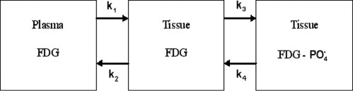
The FDG-PET based standardized uptake value of glucose in the liver was used as a surrogate for the net influx constant (K 1 ) and computed tomography perfusion measurements of combined arterial and portal perfusion as a surrogate for K 1 ( ). Thus an index of hepatic phosphorylation was obtained by the ratio of standardized uptake value and THP.
Get Radiology Tree app to read full this article<
Appendix B
Texture Analysis Methodology
Get Radiology Tree app to read full this article<
Image Filtration
Get Radiology Tree app to read full this article<
G(x,y)=e−x2+y22πσ2 G
(
x
,
y
)
=
e
−
x
2
+
y
2
2
π
σ
2
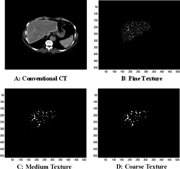
where (x, y) are the spatial coordinates of the image matrix and sigma, σ, is the standard deviation. The 2D Gaussian distribution effectively blurs the image, wiping out all structures at scales much smaller than the sigma of the Gaussian. This distribution has the desirable characteristics of being smooth and localized in both the spatial and frequency domains and is therefore less likely to introduce any changes that were not present in the original image. Thus the Gaussian distribution enables the highlighting of only hepatic textural features of a particular scale in contrast-agent enhanced CT images corresponding to a particular σ value. We have employed this filtration technique to filter out textural features of varying scale; fine scale enhances parenchyma whereas medium to coarse scale enhances blood vessels.
Get Radiology Tree app to read full this article<
Get Radiology Tree app to read full this article<
∇2G(x,y)=−1πσ4(1−x2+y22σ2)e−(x2+y22σ2) ∇
2
G
(
x
,
y
)
=
−
1
π
σ
4
(
1
−
x
2
+
y
2
2
σ
2
)
e
−
(
x
2
+
y
2
2
σ
2
)
From the mathematical expression of this circularly symmetric filter at different σ values, the number of pixels representing the width between the diametrically opposite zero-crossing points in this filter can be calculated (see Fig 5 ). The width of the filter at different σ values are obtained by evaluating the LoG spatial distribution along the x and y directions ( Table 4 ). The width can be considered as the scale at which the structures in the image will be highlighted and enhanced, whereas structures below this scale will become blurred ( Fig 1 ). The lower the sigma value, the smaller is the width of the filter in the spatial domain and the larger is the pass-band region of the filter in the frequency domain, highlighting fine details or features in the filtered image in the spatial domain. Similarly, the higher the sigma value, the higher is the width of the filter in the spatial domain; this corresponds to a smaller pass-band region of the filter in the frequency domain, highlighting coarse features in the filtered image in the spatial domain.

Table 4
Filter Sigma Value and the Corresponding Width of the Filter (Pixels and mm)
Sigma (σ) Texture Type Filter Width (Pixels) Filter Width (mm) 0.5 Fine 2 1.68 1.5 Medium 6 5.04 2.0 Coarse 10 8.40
Get Radiology Tree app to read full this article<
Get Radiology Tree app to read full this article<
Quantification of Texture
Get Radiology Tree app to read full this article<
m=1N∑(x,y)∈R[a(x,y)] m
=
1
N
∑
(
x
,
y
)
∈
R
[
a
(
x
,
y
)
]
u=∑kl=1[p(l)]2 u
=
∑
l
=
1
k
[
p
(
l
)
]
2
Besides the use of filtered fine, medium, and coarse mean gray-level intensity quantification, normalized fine, medium, and coarse mean gray-level intensities were also quantified. Normalization was done primarily to minimize the effects of the variation in CT attenuation values occurring from one patient to another and reducing the effect of noise on texture quantification. Mean gray-level intensity and uniformity for fine, medium, and coarse textures were normalized with respect to the largest observed liver texture feature highlighted by the filter (σ = 2.5, width = 12 pixels or 10.08 mm) in our study.
Normalizedfinemeangray-levelintensity=1N∑(x,y)∈R[a(x,y)σ=0.5(fine)]1N∑(x,y)∈R[a(x,y)σ=2.5(large)] N
o
r
m
a
l
i
z
e
d
f
i
n
e
m
e
a
n
g
r
a
y
-
l
e
v
e
l
i
n
t
e
n
s
i
t
y
=
1
N
∑
(
x
,
y
)
∈
R
[
a
(
x
,
y
)
σ
=
0.5
(
f
i
n
e
)
]
1
N
∑
(
x
,
y
)
∈
R
[
a
(
x
,
y
)
σ
=
2.5
(
l
a
r
g
e
)
]
Normalizedfineuniformity=∑kl=1[p(l)σ=0.5]2∑kl=1[p(l)σ=2.5]2 N
o
r
m
a
l
i
z
e
d
f
i
n
e
u
n
i
f
o
r
m
i
t
y
=
∑
l
=
1
k
[
p
(
l
)
σ
=
0.5
]
2
∑
l
=
1
k
[
p
(
l
)
σ
=
2.5
]
2
Normalizedmediummeangray-levelintensity=1N∑(x,y)∈R[a(x,y)σ=1.5(medium)]1N∑(x,y)∈R[a(x,y)σ=2.5(large)] N
o
r
m
a
l
i
z
e
d
m
e
d
i
u
m
m
e
a
n
g
r
a
y
-
l
e
v
e
l
i
n
t
e
n
s
i
t
y
=
1
N
∑
(
x
,
y
)
∈
R
[
a
(
x
,
y
)
σ
=
1.5
(
m
e
d
i
u
m
)
]
1
N
∑
(
x
,
y
)
∈
R
[
a
(
x
,
y
)
σ
=
2.5
(
l
a
r
g
e
)
]
Normalizedmediumuniformity=∑kl=1[p(l)σ=1.5]2∑kl=1[p(l)σ=2.5]2 N
o
r
m
a
l
i
z
e
d
m
e
d
i
u
m
u
n
i
f
o
r
m
i
t
y
=
∑
l
=
1
k
[
p
(
l
)
σ
=
1.5
]
2
∑
l
=
1
k
[
p
(
l
)
σ
=
2.5
]
2
Normalizedcoarsemeangray-levelintensity=1N∑(x,y)∈R[a(x,y)σ=2.0(coarse)]1N∑(x,y)∈R[a(x,y)σ=2.5(large)] N
o
r
m
a
l
i
z
e
d
c
o
a
r
s
e
m
e
a
n
g
r
a
y
-
l
e
v
e
l
i
n
t
e
n
s
i
t
y
=
1
N
∑
(
x
,
y
)
∈
R
[
a
(
x
,
y
)
σ
=
2.0
(coarse)
]
1
N
∑
(
x
,
y
)
∈
R
[
a
(
x
,
y
)
σ
=
2.5
(
l
a
r
g
e
)
]
Normalizedcoarseuniformity=∑kl=1[p(l)σ=2.0]2∑kl=1[p(l)σ=2.5]2 N
o
r
m
a
l
i
z
e
d
c
o
a
r
s
e
u
n
i
f
o
r
m
i
t
y
=
∑
l
=
1
k
[
p
(
l
)
σ
=
2.0
]
2
∑
l
=
1
k
[
p
(
l
)
σ
=
2.5
]
2
Get Radiology Tree app to read full this article<
Get Radiology Tree app to read full this article<
References
1. Tourassi G.D.: Journey towards computer-aided diagnosis: role of image texture analysis. Radiology 1999; 213: pp. 317-320.
2. Durgin F.H., Proffitt D.R.: Visual learning in the perception of texture: simple and contingent aftereffects of texture density. Spat Vis 1996; 9: pp. 424-474.
3. Folfiak P.: Forming sparse representations by local anti-Hebbian learning. Biol Cybern 1990; 64: pp. 165-170.
4. Field D.J., Hayes A., Hess R.F.: Contour integration by the human visual system: evidence for a local “association field.”. Vision Res 1993; 33: pp. 173-193.
5. Karni A., Sagi D.: The time course of learning a visual skill. Nature 1993; 365: pp. 250-252.
6. Bilello M., Gokturk S.B., Desser T., et. al.: Automatic detection and classification of hypodense hepatic lesions on contrast-enhanced venous-phase CT. Med Phys 2004; 31: pp. 2584-2593.
7. Gletsos M., Mougiakakou S.G., Metsopoulos G.K., et. al.: A computer-aided diagnostic system to characterize CT focal liver lesions: design and optimization of a neural network classifier. IEEE Trans Inf Technol Biomed 2003; 7: pp. 153-162.
8. Klein H.M., Klose K.C., Eisele T., et. al.: The diagnosis of focal liver lesions by the texture analysis of dynamic computed tomograms. [article in German] Rofo 1993; 159: pp. 10-15.
9. Kim T., Federle M.P., Baron R.L., et. al.: Discrimination of small hepatic hemangiomas from hypervascular malignant tumors smaller than 3 cm with three-phase helical CT. Radiology 2001; 219: pp. 699-706.
10. Afaq Hussain S., Shigeru E.: Use of neural networks for feature based recognition of liver region on CT images.2000.pp. 831-840.
11. Mala K., Sadasivam V.: Automatic segmentation and classification of diffused liver diseases using wavelet based texture analysis and neural network.INDICON, 2005 Annual IEEE.2005.pp. 216-219.
12. Ganeshan B, Miles KA, Young RCD, et al. Hepatic entropy and uniformity: additional parameters that can potentially increase the utility of contrast enhancement during abdominal CT. Clinical Radiology. In press.
13. Mir A.H., Hanmandlu M., Tandon S.N.: Texture analysis of CT-images for early detection of liver malignancy. Biomed Sci Instrum 1995; 31: pp. 213-217.
14. Bezy-Wendling J., Kretowski M., Rolland Y., et. al.: Towards a better understanding of texture in vascular CT scan simulated images. IEEE Trans Biomed Eng 2001; 48: pp. 120-124.
15. Dixon A.K., Walshe J.M.: Computed tomography of the liver in Wilson disease. J Comput Assist Tomogr 1984; 8: pp. 46-49.
16. Howard J.M., Ghent C.N., Carey L.S., et. al.: Diagnostic efficacy of hepatic computed tomography in the detection of body iron overload. Gastroenterology 1983; 84: pp. 209-215.
17. Ricci C., Longo R., Gioulis E., et. al.: Noninvasive in vivo quantitative assessment of fat content in human liver. J Hepatol 1997; 27: pp. 108-113.
18. Choi Y., Hawkins R.A., Huang S.C., et. al.: Evaluation of the effect of glucose ingestion and kinetic model configuration of FDG in the normal liver. J Nucl Med 1994; 35: pp. 818-823.
19. Miles K.A., Comber L., Keith C.J., et. al.: Combining perfusion CT and FDG-PET data demonstrates reduced hepatic phosphorylation of glucose in patients with advanced colorectal cancer and poor survival. Eur Radiol 2003; 13: 1:293
20. Munk O.L., Bass l., Roelsgaard K., Bender D., et. al.: Liver kinetics of glucose analogs measured in pigs by PET: importance of dual-input blood sampling. J Nucl Med 2001; 42: pp. 795-801.
21. Sadato N., Tsuchida T., Nakaumra S., et. al.: Non-invasive estimation of the net influx constant using the standardized uptake value for quantification of FDG uptake of tumors. Eur J Nucl Med 1998; 25: pp. 559-564.
22. Cuenod C.A., Leconte I., Siauve N., et. al.: Early changes in liver perfusion caused by occult metastases in rats: detection with quantitative CT. Radiology 2001; 218: pp. 556-561.
23. Kruskal J.B., Thomas P., Kane R.A., et. al.: Hepatic perfusion changes in mice livers with developing colorectal cancer metastases. Radiology 2004; 231: pp. 482-490.
24. Leen E., Angerson W.G., Cooke T.G., et. al.: Prognostic power of Doppler perfusion index in colorectal cancer. Ann Surg 1996; 223: pp. 199-203.
25. Iozzo P., Geisler F., Oikonen V., et. al.: Insulin stimulates liver glucose uptake in humans: an 18 F-FDG PET Study. J Nucl Med 2003; 44: pp. 682-689.
26. Tsushima Y., Aoki J., Endo K.: The effect of fatty infiltration on the liver tissue enhancement during portal phase computed tomography. Acad Radiol 2003; 10: pp. 1008-1012.
27. Copeland G.P., Leinster S.J., Davis J.C., et. al.: Insulin resistance in patients with colorectal cancer. Br J Surg 1987; 74: pp. 1031-1035.
28. Makino T., Noguchi Y., Yoshikawa T., et. al.: Circulating interleukin 6 concentrations and insulin resistance in patients with cancer. Br J Surg 1998; 85: pp. 1658-1662.
29. Miles K.A., Hayball M.P., Dixon A.K.: Functional images of hepatic perfusion obtained with dynamic computed tomography. Radiology 1993; 188: pp. 405-411.
30. Sydow K., Mondon C.E., Cooke J.P.: Insulin resistance: potential role of the endogenous nitric oxide synthase inhibitor ADMA. Vasc Med 2005; 10: pp. S35-S43.
31. Tsushima Y., Blomley M.J.K., Yokoyama H., et. al.: Does the presence of distant and local malignancy alter parenchymal perfusion in apparently disease-free areas of the liver?. Digest Dis Sci 2001; 46: pp. 2113-2119.
32. Platt J.F., Francis I.R., Ellis J.H., et. al.: Difference in global hepatic enhancement assessed by dynamic CT in normal subjects and patients with hepatic metastases. J Comp Assist Tomogr 1997; 21: pp. 348-354.
33. Cuenod C.A., Leconte I., Siauve N., et. al.: Early changes in liver perfusion caused by occult metastases in rats: detection with quantitative CT. Radiology 2001; 218: pp. 556-561.
34. Nanko M., Shimada H., Yamaoka H., et. al.: Micrometastatic colorectal cancer lesions in the liver. Surg Today 1998; 28: pp. 707-713.
35. Haugeberg G., Strohmeyer T., Lierse W., et. al.: The vascularisation of liver metastases. J Cancer Res Clin Oncol 1988; 114: pp. 415-419.
36. Desch C.E., Benson A.B., Somerfield M.R., et. al., American Society of Clinical Oncology: Colorectal cancer surveillance: 2005 update of an American Society of Clinical Oncology practice guideline. J Clin Oncol 2005; 23: pp. 8512-8519.
37. Tayek J.A.: A review of cancer cachexia and abnormal glucose metabolism in humans with cancer. J Am Coll Nutr 1992; 11: pp. 445-456.
38. Marr D.: Representing the image: zero-crossings and the raw primal sketch.Wilson J.Monsour P.Vision.1982.W.H. Freeman and CompanySan Francisco:pp. 54-68.