Interpreting Change in Quantitative Imaging Biomarkers

Rationale and Objectives

Quantitative imaging biomarkers (QIBs) are becoming increasingly adopted into clinical practice to monitor changes in patients’ conditions. The repeatability coefficient (RC) is the clinical cut-point used to discern between changes in a biomarker’s measurements due to measurement error and changes that exceed measurement error, thus indicating real change in the patient. Imaging biomarkers have characteristics that make them difficult for estimating the repeatability coefficient, including nonconstant error, non-Gaussian distributions, and measurement error that must be estimated from small studies.

Methods

We conducted a Monte Carlo simulation study to investigate how well three statistical methods for estimating the repeatability coefficient perform under five settings common for QIBs.

Results

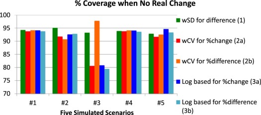
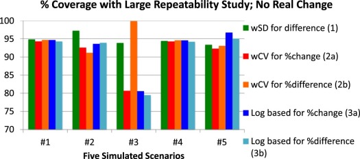
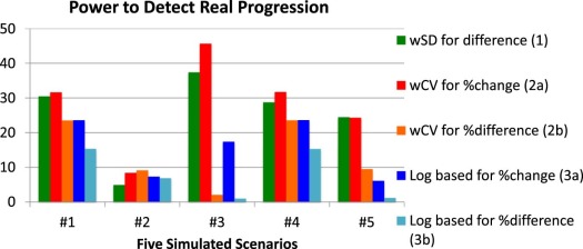
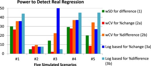
When the measurement error is constant and replicates are normally distributed, all of the statistical methods perform well. When the measurement error is proportional to the true value, approaches that use the log transformation or coefficient of variation perform similarly. For other common settings, none of the methods for estimating the repeatability coefficient perform adequately.

Conclusion

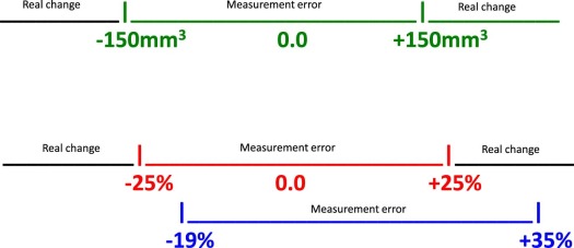
Many of the common approaches to estimating the repeatability coefficient perform well for only limited scenarios. The optimal approach depends strongly on the pattern of the within-subject variability; thus, a precision profile is critical in evaluating the technical performance of QIBs. Asymmetric bounds for detecting regression vs progression can be implemented and should be used when clinically appropriate.

Introduction

As quantitative imaging biomarkers (QIBs) become increasingly adopted into clinical practice for diagnosis, prognosis, and disease monitoring, it is critical that clinicians be able to interpret them properly. Clinicians must be able to discern between changes in a biomarker’s measurements that are expected because of measurement error by the imaging system and changes that exceed measurement error and thus indicate a real change in the patient.

Studies of the technical performance of QIBs, particularly studies of their repeatability, are used to help radiologists interpret change. Organizations such as the Quantitative Imaging Biomarker Alliance (QIBA) conduct groundwork studies to estimate biomarkers’ performance. They also perform meta-analyses to summarize biomarkers’ performance over multiple published studies . From these studies of repeatability, investigators calculate a cut-point, or threshold, for discerning when a measured change is attributable to measurement error vs when the measured change should be interpreted as a real change in the patient, with some stated degree of confidence . For illustration, when measuring the change in volume of a pulmonary lesion from baseline, a measured change <25% might be considered purely measurement error, whereas a measured change exceeding 25% might be considered a real change, with 95% confidence .

Get Radiology Tree app to read full this article<

Methods

Defining Change

Get Radiology Tree app to read full this article<

Table 1

Three Definitions of Change in QIBs \*

Difference from baseline

dˆ=(Yit−Yib) d

(

−

)

Percentage change from baseline

%dˆb=(Yit−Yib)/Yib×100 %

(

−

)

100

Percentage difference

%dˆmean=(Yit−Yib)(Yib+Yit)/2×100 %

mean

(

−

)

(

)

100

QIBs, quantitative imaging biomarkers.

Get Radiology Tree app to read full this article<

Methods for Estimating Cut-Points From Technical Performance Studies

Get Radiology Tree app to read full this article<

Yik=βo+β1Xik+ϵik, Y

where β o is the fixed bias, β 1 is the proportional bias, and ϵik ϵ

k is the measurement error. It is often assumed that the measurement error is constant and follows a normal distribution, ϵik~N(0,σ2) ϵ

(

) . We vary these assumptions in our Monte Carlo simulation study to consider scenarios typical in imaging. The measurement error, σ 2 , is often referred to as the within-subject variance. Its square root is referred to as the within-subject standard deviation (wSD) .

Get Radiology Tree app to read full this article<

σˆ2=∑Ni=1{Yi1−Yi2}2/2N, σ

∑

{

−

}

where Y ik denotes the biomarker measurement for the k th replicate on the i th subject. Assuming constant within-subject variance and normality, the cut-point associated with 95% confidence is then

RCˆ=1.96×2σˆ2−−−√, R

1.96

where RC is the repeatability coefficient, or the least significant difference between two repeat measurements taken under identical conditions . Changes in the biomarker that exceed +RC or are less than −RC are considered real changes (not as a result of just measurement error), with 95% confidence. Specifically, measured differences <−RC are considered true regression, whereas measured differences >+RC are considered true progression. We refer to this simple approach as Approach 1 (see first row of Table 2 ).

Table 2

Three Approaches to Discerning Measurement Error From Real Change

“The observed change in QIB is attributable to measurement error.” “The observed change in the QIB represents true change in the patient, with 95% confidence.” Approach 1

−RCˆ<dˆ<+RCˆ −

dˆ<−RCˆordˆ>+RCˆ d

−

Approach 2A

−%RCˆ<%dˆb<+%RCˆ −

%dˆb<−%RCˆor%dˆb>+%RCˆ %

−

Approach 2B

−%RCˆ<%dˆmean<+%RCˆ −

mean

%dˆmean<−%RCˆor%dˆmean>+%RCˆ %

mean

−

mean

Approach 3A

RClnlower<%dˆb<RClnupper R

lnlower

lnupper

%dˆb<RClnloweror%dˆb>RClnupper %

lnlower

lnupper

Approach 3B

%RClnlower<%dˆmean<%RClnupper %

lnlower

mean

lnupper

%dˆmean<%RClnloweror%dˆmean>%RClnupper %

mean

lnlower

mean

lnupper

QIB, quantitative imaging biomarker.

Get Radiology Tree app to read full this article<

wCVˆ2=∑Ni=1{(Yi1−Yi2)2/(2Y¯¯¯2i)}/N. w

∑

{

(

−

)

(

)

}

Get Radiology Tree app to read full this article<

%RCˆ=1.96×2wCVˆ2−−−−−−√ %

1.96

and the symmetric cut-points are defined as Approach 2 in Table 2 . Note that %RC could be used to define a cut-point for the percentage change from baseline ( %dˆb %

b ) or for the percentage difference ( %dˆmean %

mean ). These are presented as Approaches 2A and 2B in Table 2 , respectively.

Get Radiology Tree app to read full this article<

σˆ2ln=∑Ni=1{ln(Yi1)−ln(Yi2)}2/2N. σ

∑

{

(

)

−

(

)

}

Get Radiology Tree app to read full this article<

RCˆln=1.96×2σˆ2ln−−−−√. R

1.96

Get Radiology Tree app to read full this article<

RClnlower=(exp(−RCˆln)−1)andRClnupper=(exp(+RCˆln)−1). R

lower

(

exp

(

−

)

−

)

and

upper

(

exp

(

)

−

)

Get Radiology Tree app to read full this article<

QIB Repeatability Data

Get Radiology Tree app to read full this article<

Table 3

Assessment of the Distribution of Intra-Subject Repeated Measurements

QIB Setting No. of Observations Distribution for Intra-Subject Replicates Magnetic resonance imaging T1 values Phantom study with replicate scans of each target 15 replicates per target Close to normally distributed except for targets at low T1 values where there’s clustering at the minimum values Ultrasound shear wave speed Phantom study with replicate scans of each target 10 replicates per target Close to normally distributed Magnetic resonance elastography values Clinical study with 1 scan per subject, evaluated by multiple algorithms 10 replicates per subject Close to normally distributed except for subjects with low values where there is clustering at these low values Computed tomography acetabular angle Clinical study with 1 scan per patient, interpreted by multiple readers 4 replicates per subject Close to normally distributed

QIB, quantitative imaging biomarker.

Get Radiology Tree app to read full this article<

Monte Carlo Simulation Study

Get Radiology Tree app to read full this article<

Table 4

Five Scenarios for Monte Carlo Simulation

Scenario Description Distribution of True Value of Biomarker \* Distribution of Replicate Measurements within Subject † 1 QIB with constant wSD and normally distributed replicates_X_ ~ N (100, 100) ε ~ N (0,100) 2 QIB with constant wSD and log-normally distributed replicates_X_ ~ N (100, 100) ε = exp( Z ), where Z ~ N (0,10) 3 QIB with clustering at one extreme ‡ X ~ N (10, 100) ε ~ N (0,100), but values less than zero were set to zero 4 QIB with constant wCV and normally distributed replicates_X_ ~ N (20, 10) ε ~ N (0,σ 2 ), with σ increasing with true biomarker value: σ=(0.1)×(X) σ

(

0.1

)

(

) 5 QIB where wSD is larger for both small and large values of QIB § X ~ N (20, 10) ε ~ N (0,σ 2 ), with σ 2 = 100 for X < 17 or >23; otherwise σ 2 = 20 and values less than zero were set to zero

QIB, quantitative imaging biomarker; wCV, within-subject coefficient of variation; wSD, within-subject standard deviation.

Get Radiology Tree app to read full this article<

Results

Get Radiology Tree app to read full this article<

Scenario 1: Constant wSD and Normally Distributed Replicates

Get Radiology Tree app to read full this article<

Scenario 2: Constant wSD and Log-Normally Distributed Replicates

Get Radiology Tree app to read full this article<

Scenario 3: Clustering of Values at One Extreme

Get Radiology Tree app to read full this article<

Scenario 4: Constant wCV and Normally Distributed Replicates

Get Radiology Tree app to read full this article<

Scenario 5: “Sweet-Spot” with High wSD at Each End and Normally Distributed Replicates

Get Radiology Tree app to read full this article<

Discussion

Get Radiology Tree app to read full this article<

RCˆlower=Za×2σˆ2−−−√RCˆupper=Zb×2σˆ2−−−√. R

lower

upper

Get Radiology Tree app to read full this article<

σˆ2i=bo+b1(Y¯¯¯i), σ

(

)

where the estimated within-subject variance of subject i is a function of the mean of the measurements from subject i . A quadratic term could also be added and tested using ordinary least squares regression. The estimated regression coefficients, bˆo b

o and bˆ1 b

1 , are then used to define dynamic cut-points, that is, cut-points that vary with a future subject’s baseline measurement. For example, for the i th future subject, the cut-point associated with 95% confidence is then

RCˆdynamic=1.96×2(bˆo+bˆ1Yib)−−−−−−−−−−−√, R

dynamic

1.96

(

)

where bˆo b

o and bˆ1 b

1 are estimated from a technical performance study of a biomarker’s repeatability, Y ib is the baseline measurement for future subject i . When we evaluated this approach in our Monte Carlo simulation study with N = 35, this model approach did not have nominal coverage, with coverage of only 89%–92%. With a larger sample size ( N = 100), the coverage improved somewhat but it did not reach the nominal level. Thus, this sort of approach might be extremely useful for QIBs but much larger technical performance studies than are typically performed now would be needed.

Get Radiology Tree app to read full this article<

Acknowledgments

Get Radiology Tree app to read full this article<

References

1. Radiological Society of North America (RSNA) : Quantitative Imaging Biomarkers Alliance. Available at: www.rsna.org/QIBA/ Accessed November 20, 2017
2. Sullivan D.C., Obuchowski N.A., Kessler L.G., et. al.: Metrology standards for quantitative imaging biomarkers. Radiology 2015; 277: pp. 813-825.
3. Raunig D., McShane L.M., Pennello G., et. al.: Quantitative imaging biomarkers: a review of statistical methods for technical performance assessment. Stat Methods Med Res 2015; 24: pp. 27-67.
4. Obuchowski N.A., Reeves A.P., Huang E.P., et. al.: Quantitative imaging biomarkers: a review of statistical methods for computer algorithm comparisons. Stat Methods Med Res 2015; 24: pp. 68-106.
5. Barnhart H.X., Barboriak D.P.: Applications of the repeatability of quantitative imaging biomarkers: a review of statistical analysis of repeat data sets. Transl Oncol 2009; 2: pp. 231-235.
6. QIBA : CT Tumor Volumetry for Advanced Disease. Available at: http://qibawiki.rsna.org/index.php/Profiles Accessed November 20, 2017
7. Obuchowski N.A., Bullen J.: Quantitative imaging biomarkers: effect of sample size and bias on confidence interval coverage. Stat Methods Med Res 2017; In press
8. Bland J.M., Altman D.G.: Measuring agreement in method comparison studies. Stat Methods Med Res 1999; 8: pp. 135-160.
9. Weber W.A., Gatsonis C.A., Mozley P.D., et. al.: Repeatability of 18 F-FDG PET/CT in advanced non-small cell lung cancer: prospective assessment in 2 multicenter trials. J Nucl Med 2015; 56: pp. 1137-1143.
10. Winfield J.M., Tunariu N., Rata M., et. al.: Extracranial soft-tissue tumors: repeatability of apparent diffusion coefficient estimates from diffusion-weighted MR imaging. Radiology 2017; 284: pp. 88-99.
11. Obuchowski N.A., Barnhart H.X., Buckler A.J., et. al.: Statistical issues in the comparison of quantitative imaging biomarker algorithms using pulmonary nodule volume as an example. Stat Methods Med Res 2015; 24: pp. 107-140.
12. Lodge M.: Repeatability of SUV in oncologic 18 F-FDG PET. J Nucl Med 2017; 58: pp. 523-532.

Interpreting Change in Quantitative Imaging Biomarkers

Rationale and Objectives

Methods

Results

Conclusion

Introduction

Methods

Defining Change

Methods for Estimating Cut-Points From Technical Performance Studies

QIB Repeatability Data

Monte Carlo Simulation Study

Results

Scenario 1: Constant wSD and Normally Distributed Replicates

Scenario 2: Constant wSD and Log-Normally Distributed Replicates

Scenario 3: Clustering of Values at One Extreme

Scenario 4: Constant wCV and Normally Distributed Replicates

Scenario 5: “Sweet-Spot” with High wSD at Each End and Normally Distributed Replicates

Discussion

Acknowledgments

References

Further Reading

Breast Imaging Outcomes following Abnormal Thermography

Breast MRI as a Problem-solving Study in the Evaluation of BI-RADS Categories 3 and 4 Microcalcifications

Cardiothoracic MRI in the ICU