Learning Fourier Descriptors for Computer-Aided Diagnosis of the Supraspinatus

Rationale and Objectives

Supraspinatus muscle disorders are frequent and debilitating, resulting in pain and a limited range of shoulder motion. The gold standard for diagnosis involves an invasive surgical procedure. As part of a proposed clinical workflow for noninvasive computer-aided diagnosis (CAD) of the condition of the supraspinatus, we present a method to classify three-dimensional shapes of the muscle into relevant pathology groups, based on magnetic resonance (MR) images.

Materials and Methods

We obtained MR images of the shoulder from 72 patients, separated into five pathology groups. The imaging protocol ensures that the supraspinatus is consistently oriented relative to the MR imaging plane for each scan. Next, we compute the Fourier coefficients of two-dimensional contours lying on parallel imaging planes and integrate the corresponding frequency components across all contours. To classify the shapes, we learn the Fourier coefficients that best distinguish the different classes.

Results

We show that our method leads to significant improvement when compared to previous work. We are able to distinguish between normal shapes and shapes that possess a pathology with an accuracy of almost 100%. Moreover, we can differentiate between the different pathology groups with an average accuracy of 86%.

Conclusion

We confirm that analyzing the three-dimensional shape of the muscle has potential as a form of diagnosis reinforcement to assess the condition of the supraspinatus. Moreover, our proposed descriptor based on Fourier coefficients is able to distinguish the different pathology groups with accuracies higher than those obtained by previous work, indicating its potential application to support a system for CAD of the supraspinatus.

The supraspinatus muscle originates from the supraspinatus fossa of the scapula and runs along the top of the shoulder blade. This muscle is part of the rotator cuff, which is a group of muscles and tendons responsible for shoulder movement and stabilization. Disorders affecting the rotator cuff can cause pain and reduce patient mobility , and their occurrence is frequent, with a reported rate of 30% of individuals older than 60 years of age in a cadaveric study . Supraspinatus disorders involving tendon tearing can be accompanied by muscle retraction, atrophy, or both. The standard procedure for the diagnosis of rotator cuff disorders is shoulder arthroscopy, which is a surgery involving the insertion of an optical camera. However, diagnosis based on magnetic resonance (MR) images is a preferred noninvasive alternative. Additionally, the impact of a supraspinatus tendon tear on the overall body of the muscle has prognostic value and is visible on MR images, but is not visible during arthroscopy .

The long-term goal of our research is to develop a tool for noninvasive computer-aided diagnosis (CAD) of the supraspinatus, based on three-dimensional (3D) shapes extracted from MR images. The realization of this goal would lead to several important benefits and results. First, CAD can be helpful to provide a second opinion or to serve as a form of diagnosis reinforcement for the physician; it can also be valuable when other clinical data (eg, palpation or range-of-motion exams in the context of musculoskeletal disorders) do not provide a clear indication of the pathology. Second, understanding the relationship between shape and pathology can be helpful in providing evidence for etiological or epidemiological studies. Last, the impact of a torn tendon on the shape of the supraspinatus, which has prognostic significance, can be assessed more accurately by analyzing the 3D shape of the muscle. We are therefore motivated to perform an automated analysis of the 3D shape of the supraspinatus, which would allow us to improve on the diagnosis based on two-dimensional (2D) MR images or even shoulder arthroscopy. Previous work concluded that the shape of the supraspinatus is helpful in the diagnosis of rotator cuff disorders, but a more effective shape analysis procedure is necessary to achieve a pathology classification with 100% accuracy . From a computational viewpoint, our goal is: given a set of shapes and their diagnoses (which were determined by a physician), learn the relationship between the shape of the supraspinatus and its pathologies, and employ such a relationship in CAD.

Get Radiology Tree app to read full this article<

Open full size image

Figure 1

Input to the representation used in this work. (a) Magnetic resonance (MR) images of the shoulder of a patient are acquired (only one image is shown). (b) The three-dimensional shape of the supraspinatus muscle is segmented from the MR images. (c) The final shape of the muscle is captured as a set of two-dimensional (2D) contours (only three contours are shown for illustration purposes).

Get Radiology Tree app to read full this article<

Materials and methods

Get Radiology Tree app to read full this article<

Table 1

Pathology Groups Considered in the Study

Pathology Abbreviation Number of Shapes No pathology (normal) N 14 Tear T 19 Tear and atrophy TA 13 Tear and retraction TR 15 Tear and atrophy and retraction TAR 11

Get Radiology Tree app to read full this article<

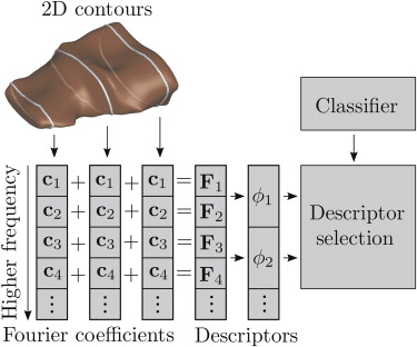
Descriptor Computation

Contour decomposition

Get Radiology Tree app to read full this article<

fk=∑N−1n=0xnexp(−2πiNkn), f

∑

−

exp

(

−

)

where k ∈ in [0, 1, …, N–1] and f is a vector of complex coefficients. The Fourier transform decomposes a signal into a set of frequency components that provide a complete, coarse-to-fine description of the signal. The coefficient f k corresponds to the amount of frequency k that is present in the original signal. The frequencies k are increasing multiples of the sampling frequency.

Get Radiology Tree app to read full this article<

Obtaining invariance

Get Radiology Tree app to read full this article<

s1fks1fl=s2fks2fl,∀k, s

∀

where f l is a specific non-zero component. Because we discard the DC-components (set | f 0 | to zero), we use the first frequency components | f 1 | for the previously mentioned scale normalization. Therefore, the normalized coefficients are given by ck=|fk|/|f1| c

| , where |f1|=maxl|fl1| |f

max

| , with flk f

l denoting the coefficient associated to frequency k for contour l in the muscle.

Get Radiology Tree app to read full this article<

Final descriptor

Get Radiology Tree app to read full this article<

F=(∑lcl1,∑lcl2,…,∑lclN−1) F

(

∑

−

)

The descriptor component F k (referred to simply as component hereafter), indicates the total contribution of frequency k to the shape, measured on slices along a specific axis. The resolution within each slice is between 0.3 and 0.6 mm, so the frequencies analyzed are multiples of the sampling frequency, ie k106 k

6 to k103 k

3 cycles/mm. Because the contours lie on planes aligned in a consistent direction in all shapes and they are described by rotation-, translation-, and scale-invariant components, the final descriptor F is coherent across different shapes and hence the need to establish point correspondence is avoided. The descriptor implicitly captures the 3D shape of the muscle by recording the changes in scale between the contours of a given muscle and also the variations in the shapes of the contours at different frequencies. These frequency variations are integrated for all the contours in the muscle.

Get Radiology Tree app to read full this article<

Descriptor Selection and Classification

Get Radiology Tree app to read full this article<

Partitioning and set combination

Get Radiology Tree app to read full this article<

distH(A,B)=maxa∈Aminb∈Bdist(a, b) dis

(

)

max

∈

min

∈

dist

(a, b)

where A and B are two contours, a and b are vertices on the contours, and dist(a,b) is the Euclidean distance between two vertices.

Get Radiology Tree app to read full this article<

Classification

Get Radiology Tree app to read full this article<

Multiclass scenario

Get Radiology Tree app to read full this article<

δ=argmaxi∑j,j≠ipij, δ

arg

max

∑

≠

where p ij is the posterior probability that the shape belongs to class i according to the classifier trained to distinguish between classes i and j . In this work, 1 < i < 5 and 1 < j < 5.

Get Radiology Tree app to read full this article<

Results

Get Radiology Tree app to read full this article<

Rij=TPijTPij+FNij,Pij=TPijTPij+FPij,andFij=2RijPijRij+Pij. R

and

When considering only two classes, we have that the recall R ij is also known as the sensitivity for class i , whereas the recall R ji is the specificity for class i . Moreover, the F-measure is a way of combining into a single number the recall and precision values. Because we are performing pairwise classification, we compute the average of the F-measure for the two classes involved, denoting it as Fij¯¯¯¯=(Fij+Fji)/2 F

(

)

2 . An assessment of the overall classification is given by the G-mean, which is the geometric mean of recall values for all classes. It is formally defined as

G=(∏Ki=1∏Kj=1,j≠iRij)1/(K(K−1)), G

(

∏

≠

)

(

−

)

where K is the number of classes.

Get Radiology Tree app to read full this article<

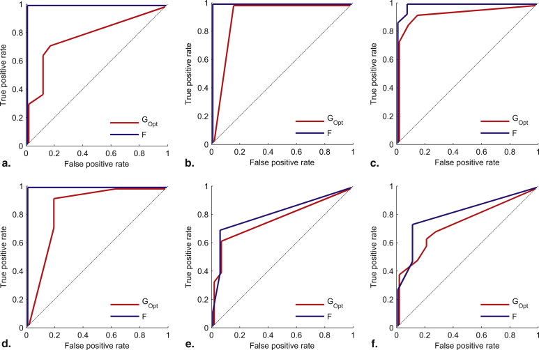
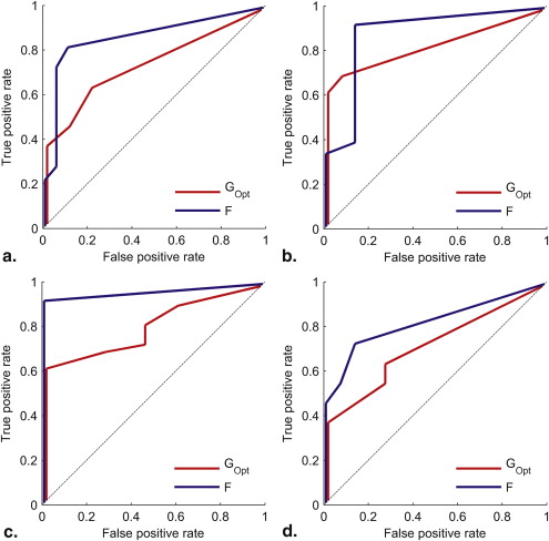
Pairwise Classification

Get Radiology Tree app to read full this article<

Table 2

Accuracy (Aij) Results for Pairwise Classification

G G Opt F N T TA TR N T TA TR N T TA TR T 70 79 100 TA 81 72 85 81 100 84 TR 79 44 82 90 65 82 97 82 89 TAR 76 73 50 73 88 73 67 73 100 87 92 81

Improvements in relation to G are marked with red color. Please refer to Table 1 for the meaning of the row and column labels.

Table 3

Recall (R ij ) Results for Pairwise Classification

G Opt F N T TA TR TAR N T TA TR TAR N 64 93 93 93 100 100 100 100 T 89 95 68 79 100 95 89 89 TA 77 62 62 54 100 69 92 100 TR 87 60 100 100 93 73 87 87 TAR 82 64 82 36 100 82 82 73

Improvements in relation to G Opt are marked with red color. Please refer to Table 1 for the meaning of the row and column labels.

Table 4

Precision (P ij ) Results for Pairwise Classification

G Opt F N T TA TR TAR N T TA TR TAR N 82 81 87 87 100 100 93 100 T 77 78 68 79 100 82 81 89 TA 91 89 100 78 100 90 86 87 TR 93 60 75 68 100 85 93 81 TAR 90 64 60 100 100 82 100 80

Improvements in relation to G Opt are marked with red color. Please refer to Table 1 for the meaning of the row and column labels.

Table 5

Average F-measure (F ij ) and G-mean Results for Pairwise Classification

G Opt F N T TA TR N T TA TR T 77 100 TA 85 79 100 83 TR 90 64 81 97 82 89 TAR 88 71 66 67 100 86 91 80 G-mean = 75 G-mean = 90

Improvements in relation to G Opt are marked with red color. Please refer to Table 1 for the meaning of the row and column labels.

Table 6

Area under ROC Curve (AUC ij ) Results for Pairwise Classification

G Opt F N T TA TR N T TA TR T 79 100 TA 93 78 100 81 TR 95 75 83 99 81 88 TAR 87 75 81 72 100 87 96 82

Improvements in relation to G Opt are marked with red color. Please refer to Table 1 for the meaning of the row and column labels.

Get Radiology Tree app to read full this article<

Multiclass Scenario

Get Radiology Tree app to read full this article<

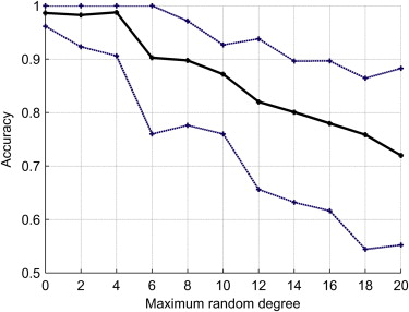
Robustness to Misalignments

Get Radiology Tree app to read full this article<

Timing

Get Radiology Tree app to read full this article<

Discussion

Pairwise Classification

Get Radiology Tree app to read full this article<

Multiclass Scenario

Get Radiology Tree app to read full this article<

Robustness to Misalignments

Get Radiology Tree app to read full this article<

Selected Descriptors

Get Radiology Tree app to read full this article<

Conclusion and future work

Get Radiology Tree app to read full this article<

References

1. Fuchs S., Chylarecki C., Langenbrinck A.: Incidence and symptoms of clinically manifest rotator cuff lesions. Int J Sports Med 1999; 20: pp. 201-205.
2. Lehman C., Cuomo F., Kummer F.J., et. al.: The incidence of full thickness rotator cuff tears in a large cadaveric population. Bull Hosp Jt Dis 1995; 54: pp. 30-31.
3. Zanetti M., Gerber C., Hodler J.: Quantitative assessment of the muscles of the rotator cuff with magnetic resonance imaging. Invest Radiol 1998; 33: pp. 163-170.
4. Morag Y., Jacobson J.A., Miller B., et. al.: MR imaging of rotator cuff injury: what the clinician needs to know. Radiographics 2006; 26: pp. 1045-1065.
5. Ward A., Hamarneh G., Ashry R., et. al.: 3D shape analysis of the supraspinatus muscle: a clinical study of the relationship between shape and pathology. Acad Radiol 2007; 14: pp. 1229-1241.
6. Ashburner J., Csernansk J.G., Davatzikos C., et. al.: Computer-assisted imaging to assess brain structure in healthy and diseased brains. Lancet Neurol 2003; 2: pp. 79-88.
7. Wang L., Swank J.S., Glick I.E., et. al.: Changes in hippocampal volume and shape across time distinguish dementia of the Alzheimer type from healthy aging. NeuroImage 2003; 20: pp. 667-682.
8. Gutman B., Wang Y., Lui L.M., et. al.: Hippocampal surface analysis using spherical harmonic function applied to surface conformal mapping. Int Conf Pattern Recognition 2006; 3: pp. 964-967.
9. Chung M.K., Nacewicz B.M., Wang S., et. al.: Amygdala surface modeling with weighted spherical harmonics. Lect Notes Computer Sci 2008; 5128: pp. 177-184.
10. Nain D., Styner M., Niethammer M., et. al.: Statistical shape analysis of brain structures using spherical wavelets. Int Symp Biomed Imaging 2007; 1: pp. 209-212.
11. Wang S., Chung M.K., Dalton K.M., et. al.: Automated diagnosis of autism using Fourier series expansion of corpus callosum boundary. Human Brain Mapping Conf 2007; 1:
12. Chen S.Y.Y., Lestrel P.E., Kerr W.J.S., et. al.: Describing shape changes in the human mandible using elliptical Fourier functions. Eur J Orthodont 2000; 22: pp. 205-216.
13. Tsai A., Wells W.M., Warfield S.K., et. al.: An EM algorithm for shape classification based on level sets. Med Image Anal 2005; 9: pp. 491-502.
14. Heimann T., Meinzer H.- P.: Statistical shape models for 3D medical image segmentation: a review. Med Image Anal 2009; 13: pp. 543-563.
15. Gotsman C., Gu X., Sheffer A.: Fundamentals of spherical parameterization for 3D meshes. ACM Trans Graphics (Proc. SIGGRAPH) 2003; 22: pp. 358-363.
16. Staib H., Duncan J.S.: Boundary finding with parametrically deformable models. Trans Patt Anal Machine Intell 1992; 14: pp. 1061-1075.
17. Hamarneh G., Gustavsson T.: Statistically constrained snake deformations. Proc Int Conf Syst Man Cybernetics 2000; 3: pp. 1610-1615.
18. Lehtinen J.T., Tingart M.J., Apreleva M., et. al.: Practical assessment of rotator cuff muscle volumes using shoulder MI. Acta Orthop Scand 2003; 74: pp. 722-729.
19. Tingart M.J., Apreleva M., Lehtinen J.T., et. al.: Shoulder magnetic resonance imaging in quantitative analysis of rotator cuff muscle volume. Clin Orthopaed Related Res 2003; 415: pp. 104-110.
20. Robertson P.L., Schweitzer M.E., Mitchell D.G., et. al.: Rotator cuff disorders: Interobserver and intraobserver variation in diagnosis with MR imaging. Radiology 1995; 194: pp. 831-835.
21. Turk G., O’Brien J.F.: Shape transformation using variational implicit functions. Proc ACM SIGGRAPH 1999; 1: pp. 335-342.
22. Wu T.-F., Lin C.-J., Weng R.C.: Probability estimates for multi-class classification by pairwise coupling. J Machine Learn Res 2004; 5: pp. 975-1005.
23. Guyon I., Elisseeff A.: An introduction to variable and feature selection. J Machine Learn Res 2003; 3: pp. 1157-1182.
24. Vapnik V.: Statistical Learning Theory.1998.WileyNew York
25. Sun Y., Kamel M.S., Wang Y., et. al.: Boosting for learning multiple classes with imbalanced class distribution. Proc. Int Conf Data Mining 2006; 1: pp. 592-602.
26. Fawcett T.: An introduction to ROC analysis. Pattern Recognit Lett 2006; 27: pp. 861-874.
27. Sokolova M.: Assessing invariance properties of evaluation measures. Proc NIPS Workshop on Testing Deployable Learning and Decision Systems 2006;
28. Skurichina M., Verzakov S., Paclik P., et. al.: Effectiveness of spectral band selection/extraction techniques for spectral data. Lecture Notes Computer Sci 2006; 4109: pp. 541-550.

Learning Fourier Descriptors for Computer-Aided Diagnosis of the Supraspinatus

Rationale and Objectives

Materials and Methods

Results

Conclusion

Materials and methods

Descriptor Computation

Contour decomposition

Obtaining invariance

Final descriptor

Descriptor Selection and Classification

Partitioning and set combination

Classification

Multiclass scenario

Results

Pairwise Classification

Multiclass Scenario

Robustness to Misalignments

Timing

Discussion

Pairwise Classification

Multiclass Scenario

Robustness to Misalignments

Selected Descriptors

Conclusion and future work

References

Further Reading

CADe Prompts and Observer Performance

CT Colonography Computer-Aided Polyp Detection

Curriculum Development For Medical Education A Six-Step Approach, 2nd Edition