
Rationale and Objectives
The purpose of this study was to characterize analytic performance of software-aided arterial vessel structure measurements across a range of scanner settings for computed tomography angiography where ground truth is known. We characterized performance for measurands that may be efficiently measured for clinical cases without use of software, as well as those that may be done manually but which is generally not done due to the effort level required unless software is employed.
Materials and Methods
Four measurands (lumen area, stenosis, wall area, wall thickness) were evaluated using tissue-mimicking phantoms to estimate bias, heteroscedasticity, and limits of quantitation both pooled across scanner settings and individually for eight different settings. Reproducibility across scanner settings was also estimated.
Results
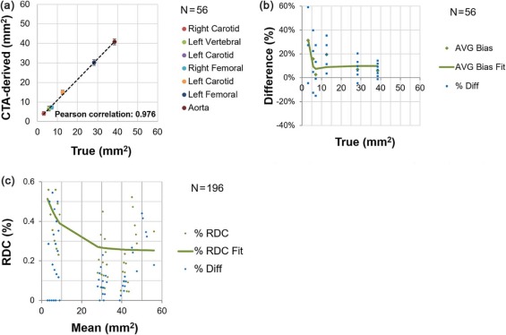
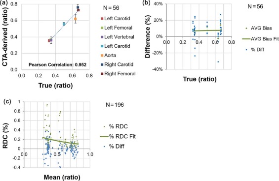
Measurements of lumen area have a near constant bias of +1.3 mm for measurements ranging from 3 mm 2 to 40 mm 2 ; stenosis bias is +7% across a 30%–70% range; wall area bias is +14% across a 50–450 mm 2 range; and wall thickness bias is +1.2 mm across a 3–9 mm range. All measurements possess properties that make them suitable for measuring longitudinal change. Lumen area demonstrates the most sensitivity to scanner settings (bias from as low as +.1 mm to as high as +2.7 mm); wall thickness demonstrates negligible sensitivity.
Conclusions
Variability across scanner settings for lumen measurands was generally higher than bias for a given setting. The converse was true for the wall measurands, where variability due to scanner settings was very low. Both bias and variability due to scanner settings of vessel structure were within clinically useful levels.
Introduction
Assessment of atherosclerotic plaque is an essential diagnostic and treatment-planning tool. Extensive efforts have begun to provide quantitative information to the physician in assessing an individual patient’s immediate cardiovascular risk. Sophisticated and powerful, post-processing of computed tomography (CT) and magnetic resonance imaging has been proposed , and this technology offers noninvasive alternatives to invasive catheterization procedures.
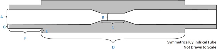
To evaluate an image-based analysis, performance should be compared to ground truth evaluated across a spectrum of disease and imaging protocols routinely used in clinical practice. In this work, we use synthetic vessel phantoms with readily measured ground truth values. The phantoms are fabricated using vessel tissue-mimicking material, as the true vessel wall thickness value in excised tissue would be difficult to ascertain, and bias is not expected to differ with clinical data. Our group has also conducted reader variability studies using clinical data to study precision based on the assumption that patient anatomy variability contributes significantly to the variability in the measurements. Our use of phantoms to estimate bias, and clinical data to estimate variability, is based on this rationale.
Materials and Methods
Get Radiology Tree app to read full this article<
Get Radiology Tree app to read full this article<
Get Radiology Tree app to read full this article<
Get Radiology Tree app to read full this article<
Imaging
Get Radiology Tree app to read full this article<
Get Radiology Tree app to read full this article<
Target Definition and Analysis
Get Radiology Tree app to read full this article<
Target Initialization
Get Radiology Tree app to read full this article<
Lumen Segmentation
Get Radiology Tree app to read full this article<
Wall Segmentation
Get Radiology Tree app to read full this article<
Segmentation Editing
Get Radiology Tree app to read full this article<
Get Radiology Tree app to read full this article<
Get Radiology Tree app to read full this article<
Quantitative Measurements
Get Radiology Tree app to read full this article<
Get Radiology Tree app to read full this article<
Statistical Analysis
Get Radiology Tree app to read full this article<
Get Radiology Tree app to read full this article<
Get Radiology Tree app to read full this article<
Get Radiology Tree app to read full this article<
Get Radiology Tree app to read full this article<
Get Radiology Tree app to read full this article<
RDC=1.962σ2ε−−−√=2.77σε R
D
C
=
1.96
2
σ
ε
2
=
2.77
σ
ε
where σ2ε σ
ε
2 is the within-vessel across-settings variance. The range in which two measurements on the same vessel were expected to fall for 95% of measurements is given by [−RDC, +RDC] . Additionally, the within-vessel coefficient of variability (wCV inter-settings ) was calculated as a measure of precision for single measurements but which may be taken according to different acquisition settings . It was calculated in an analogous fashion, but dividing each vessel-based σ2ε σ
ε
2 by the square of the mean of the two measurements. Both wCV inter-settings and %RDC are relative measures proportional to the magnitude of the vessel’s size. Because we were interested in how the metrics changed for differing vessel sizes, we plotted the percentage metrics as a function of vessel size.
Get Radiology Tree app to read full this article<
Results
Get Radiology Tree app to read full this article<
Lumen Area
Get Radiology Tree app to read full this article<
Get Radiology Tree app to read full this article<
Get Radiology Tree app to read full this article<
Table 1
(A) Bias Profile for Lumen Area Across Arteries and Scanner Settings, and (B) Stratified Analysis for Lumen Area
(A) Pooled Across Arteries and Scanner Settings True value (mm 2 ) 3.14–5.7 7.0–13.0 28.0–39.0 Overall No. of observations 16 24 16 56 Mean bias \* [95% CI] 0.94 [0.16, 1.73] 0.94 [0.25, 1.62] 2.14 [1.04, 3.23] 1.28 [0.81, 1.76] Mean % bias † [95% CI] 23.6% [4.1%, 43.1%] 8.2% [1.4%, 15.0%] 6.5% [3.1%, 9.9%] 12.1% [5.9%, 18.3%] SD [95% CI] 1.48 [1.09, 2.29] 1.62 [1.26, 2.27] 2.06 [1.52, 3.18] 1.77 [1.49, 2.18]
(B) Pooled Across Arteries But Stratified By Scanner Settings kVp 100 100 100 100 120 120 120 120 mAs 156 156 325 325 156 156 606 606 CTDIvol (mGy) ‡ 4.95 4.95 10.3 10.3 8.12 8.12 16.9 16.88 Filter B30f soft B30f B30f soft B30f B26f B30f B30f I30f Mean bias \* [95% CI] 1.10 [0.68, 2.89] 1.96 [0.25, 3.67] 0.25 [0.73, 1.22] 0.10 [−65, 0.86] 0.96 [−0.53, 2.46] 2.67 [0.63, 4.72] 2.67 [1.68, 3.66] 0.53 [−0.92, 1.99] Mean % bias † [95% CI] 11% [14%, 36%] 15% [7%, 24%] −2% [−11%, 7%] 1% [−4%, 6%] 7% [9%, 51%] 30% [9%, 51%] 36% [−1.2%, 73%] −1% [−11%, 8%] SD [95% CI] 1.93 [1.24, 4.25] 1.85 [1.19, 4.07] 1.05 [0.68, 2.32] 0.81 [0.52, 1.79] 1.62 [1.04, 3.56] 2.21 [1.42, 4.87] 1.07 [0.69, 2.36] 1.57 [1.01, 3.46]
CI, confidence interval; CTA, computed tomography angiography; DICOM, Digital Imaging and Communications in Medicine; SD, standard deviation.
The bins were established according to approximate consistency observed in result (the vertebral and the smallest carotid being the first bin, the other carotids and the smallest femoral in the middle bin, and the larger femoral with the aorta in the third bin).
Get Radiology Tree app to read full this article<
Get Radiology Tree app to read full this article<
Get Radiology Tree app to read full this article<
Get Radiology Tree app to read full this article<
Get Radiology Tree app to read full this article<
Get Radiology Tree app to read full this article<
Maximum Stenosis
Get Radiology Tree app to read full this article<
Get Radiology Tree app to read full this article<
Get Radiology Tree app to read full this article<
Table 2
(A) Bias Profile for Maximum Stenosis Across Arteries and Scanner Settings, and (B) Stratified Analysis for Maximum Stenosis
(A) Pooled Across Arteries and Scanner Settings True value (ratio) 0.32–0.35 0.50 0.63–0.67 Overall No. of observations 24 8 24 56 Mean bias \* [95% CI] 0.022 [0.007, 0.037] 0.059 [0.037, 0.081] 0.045 [0.016, 0.075] 0.037 [0.023, 0.052] Mean % bias † [95% CI] 6.48 [2.08, 10.88] −11.87 [7.47, 16.26] 6.77 [2.26, 11.29] 7.38 [4.69, 10.06] SD [95% CI] 0.036 [0.028, 0.050] 0.026 [0.017 0.053] 0.070 [0.054, 0.098] 0.054 [0.045, 0.066]
(B) Pooled Across Arteries But Stratified By Scanner Settings kVp 100 100 100 100 120 120 120 120 mAs 156 156 325 325 156 156 606 606 CTDIvol (mGy) ‡ 4.95 4.95 10.3 10.3 8.12 8.12 16.9 16.88 Filter B30f soft B30f B30f soft B30f B26f B30f B30f I30f Mean bias \* [95% CI] 0.04 [0.01, 0.07] 0.03 [0.02, 0.07] 0.04 [0.00, 0.09] 0.06 [0.00, 0.16] 0.06 [0.02, 0.10] 0.05 [0.00, 0.09] −0.01 [−0.10, 0.07] −0.01 [−0.10, 0.07] Mean % bias † [95% CI] 9% [2%, 16%] 5% [−5%, 16%] 8% [3%, 14%] 10% [1%, 19%] 12% [6%, 18%] 9% [1%, 18%] −2% [−18%, 14%] −5% [2%, 3%] SD [95% CI] 0.03 [0.02, 0.06] 0.05 [0.03, 0.11] 0.04 [0.03, 0.10] 0.06 [0.04, 0.14] 0.04 [0.02, 0.09] 0.04 [0.03, 0.09] 0.09 [0.06, 0.21] 0.02 [0.02, 0.05]
CI, confidence interval; CTA, computed tomography angiography; DICOM, Digital Imaging and Communications in Medicine; SD, standard deviation.
The bins were established according to approximate consistency observed in result (the vertebral and the two smallest carotids being the first bin, the other carotid and the smallest femoral in the middle bin, and the larger femoral with the aorta in the third bin).
Get Radiology Tree app to read full this article<
Get Radiology Tree app to read full this article<
Get Radiology Tree app to read full this article<
Get Radiology Tree app to read full this article<
Get Radiology Tree app to read full this article<
Get Radiology Tree app to read full this article<
Get Radiology Tree app to read full this article<
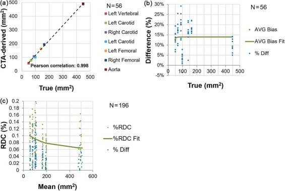
Wall Area
Get Radiology Tree app to read full this article<
Get Radiology Tree app to read full this article<
Get Radiology Tree app to read full this article<
Table 3
(A) Bias Profile for Wall Area Across Arteries and Scanner Settings, and (B) Stratified Analysis for Wall Area
(A) Pooled Across Arteries and Scanner Settings True value (mm) 50.5–67.3 89.2–98.6 140–449 Overall No. of observations 16 16 24 56 Mean bias \* [95% CI] 8.90 [6.9, 10.9] 10.4 [5.7, 15.1] 32.89 [27.3, 38.5] 19.6 [15.5, 23.7] Mean % bias † [95% CI] 14.8% [12.2%, 17.5%] 11.5% [6.2%, 16.8%] 14.8% [12.6%, 16.9%] 13.9% [12.0%, 15.7%] SD [95% CI] 3.73 [2.76, 5.77] 8.84 [6.53, 13.69] 13.19 [10.25, 18.51] 15.3 [12.9, 18.8]
(B) Pooled Across Arteries But Stratified By Scanner Settings kVp 100 100 100 100 120 120 120 120 mAs 156 156 325 325 156 156 606 606 CTDIvol (mGy) ‡ 4.95 4.95 10.3 10.3 8.12 8.12 16.9 16.88 Filter B30f soft B30f B30f soft B30f B26f B30f B30f I30f Mean bias \* [95% CI] 19.84 [−0.37, 40.05] 17.24 [0.40, 34.08] 17.91 [6.64, 29.18] 19.15 [8.10, 30.21] 25.87 [9.21, 42.53] 17.10 [8.04, 26.15] 20.21 [9.82, 30.61] 14.40 [1.51, 27.29] Mean % bias † [95% CI] 11% [6%, 17%] 11% [5%, 17%] 13% [8%, 19%] 15% [9%, 20%] 19% [11%, 26%] 14% [7%, 21%] 17% [10%, 24%] 10% [4%, 16%] SD [95% CI] 21.85 [14.08, 48.13] 18.21 [11.73, 40.10] 12.19 [7.85, 26.83] 11.95 [7.70, 26.32] 18.02 [11.61, 39.68] 9.79 [6.31, 21.55] 11.24 [7.24, 24.75] 13.94 [8.98, 30.69]
CI, confidence interval; CTA, computed tomography angiography; DICOM, Digital Imaging and Communications in Medicine; SD, standard deviation.
The bins were established according to approximate consistency observed in result (the vertebral and the smallest carotid being the first bin, the other carotids in the middle bin, and the two femorals with the aorta in the third bin).
Get Radiology Tree app to read full this article<
Get Radiology Tree app to read full this article<
Get Radiology Tree app to read full this article<
Get Radiology Tree app to read full this article<
Get Radiology Tree app to read full this article<
Get Radiology Tree app to read full this article<
Get Radiology Tree app to read full this article<
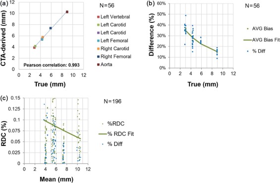
Maximum Wall Thickness
Get Radiology Tree app to read full this article<
Get Radiology Tree app to read full this article<
Get Radiology Tree app to read full this article<
Table 4
(A) Bias Profile for Maximum Wall Thickness Across Arteries and Scanner Settings, and (B) Stratified Analysis for Maximum Wall Thickness
(A) Pooled Across Arteries and Scanner Settings True value (mm) 2.88–3.05 4.3–4.43 5.88–8.96 Overall No. of observations 16 24 16 56 Mean bias \* [95% CI] 1.07 [0.98, 1.15] 1.17 [1.06, 1.29] 1.398 [1.27, 1.52] 1.21 [1.14, 1.28] Mean % bias † [95% CI] 36.0% [−33.0%, −38.9%] 26.9% [24.4%, 29.5%] 19.9% [16.7%, 23.1%] 27.5% [25.3%, 30.0%] SD [95% CI] 0.173 [0.127, 0.267] 0.268 [0.208, 0.376] 0.233 [0.172, 0.360] 0.264 [0.223, 0.325]
(B) Pooled Across Arteries But Stratified By Scanner Settings kVp 100 100 100 100 120 120 120 120 mAs 156 156 325 325 156 156 606 606 CTDIvol (mGy) ‡ 4.95 4.95 10.3 10.3 8.12 8.12 16.9 16.88 Filter B30f soft B30f B30f soft B30f B26f B30f B30f I30f Mean bias \* [95% CI] 1.20 [0.93, 1.48] 1.32 [1.12, 1.53] 1.21 [1.07, 1.35] 1.20 [0.98, 1.42] 1.39 [1.13, 1.65] 1.09 [0.78, 1.41] 1.16 [0.86, 1.45] 1.08 [0.89, 1.28] Mean % bias † [95% CI] 27% [21%, 33%] 30% [22%, 38%] 28% [20%, 36%] 27% [20%, 35%] 32% [22%, 41%] 25% [17%, 36%] 26% [18%, 35%] 25% [17%, 33%] SD [95% CI] 0.30 [0.19, 0.65] 0.22 [0.14, 0.48] 0.15 [0.10, 0.33] 0.24 [0.15, 0.52] 0.28 [0.18, 0.62] 0.34 [0.22, 0.75] 0.31 [0.20, 0.69] 0.21 [0.13, 0.46]
CI, confidence interval; CTA, computed tomography angiography; DICOM, Digital Imaging and Communications in Medicine; SD, standard deviation.
The bins were established according to approximate consistency observed in result (the vertebral and the smallest carotid being the first bin, the other carotids and the smallest femoral in the middle bin, and the larger femoral with the aorta in the third bin).
Get Radiology Tree app to read full this article<
Get Radiology Tree app to read full this article<
Get Radiology Tree app to read full this article<
Get Radiology Tree app to read full this article<
Get Radiology Tree app to read full this article<
Get Radiology Tree app to read full this article<
Get Radiology Tree app to read full this article<
Discussion
Get Radiology Tree app to read full this article<
Lumen Area
Get Radiology Tree app to read full this article<
Get Radiology Tree app to read full this article<
Maximum Stenosis
Get Radiology Tree app to read full this article<
Get Radiology Tree app to read full this article<
Wall Area
Get Radiology Tree app to read full this article<
Get Radiology Tree app to read full this article<
Maximum Wall Thickness
Get Radiology Tree app to read full this article<
Y−βoˆ±1.96×wSDˆ Y
−
β
o
±
1.96
×
w
S
D
where Y is the CTA-derived measurement for a new patient, βˆo β
o is an estimate of the constant bias, and wSD is the within-subject SD. We simulated data (ie, Y values) using the point estimates for the quadratic, linear, and intercept terms from the fitted model with the phantom data. From these data, we estimated βˆo β
o (ignoring nonlinear effects and assuming a linear slope of one). Next, we simulated data for new patients using the same point estimates for the quadratic, linear, and intercept terms from the fitted model with the phantom data. Finally, we determined the proportion of simulated patients whose 95% CI contains the true wall thickness value. The coverage of the 95% CIs for a new patient’s true wall thickness was at the nominal level, that is, 94.8%. In a second set of simulations, we evaluated the effect of the bias on the estimation of a new patient’s change in wall thickness measurements. Specifically, we evaluated the coverage of 95% CIs for a new patient’s true change in wall thickness. We used the following formula for constructing a 95% CI for the change:
(Y2−Y1)±1.96×{2(wSDˆ)2−−−−−−−−√} (
Y
2
−
Y
1
)
±
1.96
×
{
2
(
w
S
D
)
2
}
Get Radiology Tree app to read full this article<
Get Radiology Tree app to read full this article<
Get Radiology Tree app to read full this article<
Get Radiology Tree app to read full this article<
Get Radiology Tree app to read full this article<
Get Radiology Tree app to read full this article<
Acknowledgments
Get Radiology Tree app to read full this article<
Get Radiology Tree app to read full this article<
References
1. Zavodni A.E.H., Wasserman B.A., McClelland R.L., et. al.: Carotid artery plaque morphology and composition in relation to incident cardiovascular events: the Multi-Ethnic Study of Atherosclerosis (MESA). Radiology 2014; 271: pp. 381-389.
2. Puchner S.B., Liu T., Mayrhofer T., et. al.: High-risk plaque detected on coronary CT angiography predicts acute coronary syndromes independent of significant stenosis in acute chest pain: results from the ROMICAT-II Trial. J Am Coll Cardiol 2014; 64: pp. 684-692.
3. Hermann D.M., Gronewold J., Lehmann N., et. al.: Coronary artery calcification is an independent stroke predictor in the general population. Stroke 2013; 44: pp. 1008-1013. Epub 2013 Feb 28
4. Joshi F.R., Lindsay A.C., Obaid D.R., et. al.: Non-invasive imaging of atherosclerosis. Eur Heart J Cardiovas Imaging 2012; 13: pp. 205-218.
5. Muntendam P., McCall C., Sanz J., et. al.: The BioImage Study: novel approaches to risk assessment in the primary prevention of atherosclerotic cardiovascular disease—study design and objectives. Am Heart J 2010; 160: pp. 49-57. e1
6. Bae K.T.: Intravenous contrast medium administration and scan timing at CT: considerations and approaches. Radiology 2010; 256: pp. 32-61.
7. Yushkevich P.A., Piven J., Hazlett H.C., et. al.: User-guided 3D active contour segmentation of anatomical structures: significantly improved efficiency and reliability. Neuroimage 2006; 31: pp. 1116-1128.
8. Otsu N.: A threshold selection method from gray-level histograms. IEEE Trans. Sys., Man., Cyber 1979; 9: pp. 62-66.
9. Caselles V., Kimmel R., Sapiro G.: Geodesic active contours. Int J Comp Vision 1997; 22: pp. 61-97.
10. Malladi R., Sethian J.A.: Flows under min/max curvature and mean curvature. Graph Models Image Proc 1996; 58: pp. 127-141.
11. Canny J.: A computational approach to edge detection. IEEE Trans. Pattern Anal Machine Intel 1986; 8: pp. 679-698.
12. Kessler L.G., Barnhart H.X., Buckler A.J., et. al.: The emerging science of quantitative imaging biomarkers terminology and definitions for scientific studies and regulatory submissions. Stat Methods Med Res 2015; 24: pp. 9-26. Epub 2014 Jun 11
13. Obuchowski N.A., Reeves A.P., Huang E.P., et. al.: Quantitative imaging biomarkers: a review of statistical methods for computer algorithm comparisons. Stat Methods Med Res 2015; 24: pp. 68-106.
14. Algorithm Comparison Working Group: Quantitative imaging biomarkers: a review of statistical methods for computer algorithm comparisons. Stat Methods Med Res 2015; 24: pp. 68-106. Epub 2014 Jun 11
15. Case Example Working Group: Statistical issues in the comparison of quantitative imaging biomarker algorithms using pulmonary nodule volume as an example. Stat Methods Med Res 2015; 24: pp. 107-140. Epub 2014 Jun 11
16. QIBA Performance Working Group: Review of statistical methods for technical performance assessment. Stat Methods Med Res 2015; 24: pp. 27-67. Epub 2014 Jun 11
17. Barnhart H.X., Barboriak D.P.: Applications of the repeatability of quantitative imaging biomarkers: a review of statistical analysis of repeat data sets. Transl Oncol 2009; 2: pp. 231-235.
18. Mac Ananey O., Mellotte G., Maher V.: Comparison of semi-automated and manual measurements of carotid intima-media thickening. Biomed Res Int 2014; 2014: pp. 4.
19. Bianchini E., Bozec E., Gemignani V., et. al.: Assessment of carotid stiffness and intima-media thickness from ultrasound data: comparison between two methods. J Ultrasound Med 2010; 29: pp. 1169-1175.
20. Ludwig M., Zielinski T., Schremmer D., et. al.: Reproducibility of 3-dimensional ultrasound readings of volume of carotid atherosclerotic plaque. Cardiovasc Ultrasound 2008; 6: pp. 42.
21. Sun J., Zhao X.Q., Balu N., et. al.: Carotid magnetic resonance imaging for monitoring atherosclerotic plaque progression: a multicenter reproducibility study. Int J Cardiovasc Imaging 2015; 31: pp. 95-103. Published online 2014 Sep 13
22. Alizadeh Dehnavi R., Doornbos J., Tamsma J.T., et. al.: Assessment of the carotid artery by MRI at 3T: a study on reproducibility. J Magn Reson Imaging 2007; 25: pp. 1035-1043.
23. Saam T., Kerwin W.S., Chu B., et. al.: Sample size calculation for clinical trials using magnetic resonance imaging for the quantitative assessment of carotid atherosclerosis. J Cardiovasc Magn Reson 2005; 7: pp. 799-808.
24. Duivenvoorden R., de Groot E., Elsen B.M., et. al.: In vivo quantification of carotid artery wall dimensions: 3.0-Tesla MRI versus B-mode ultrasound imaging. Circ Cardiovascular Imaging 2009; 2: pp. 235-242.
25. Wasserman B.A., Astor B.C., Richey Sharrett A., et. al.: MRI measurements of carotid plaque in the atherosclerosis risk in communities (ARIC) study: methods, reliability and descriptive statistics. J Magn Reson Imaging 2010; 31: pp. 406-415.
26. Kwee R.M., Teule G.J., van Oostenbrugge R.J., et. al.: Multimodality imaging of carotid artery plaques: 18F-fluoro-2-deoxyglucose positron emission tomography, computed tomography, and magnetic resonance imaging. Stroke 2009; 40: pp. 3718-3724.
27. de Weert T.T., Ouhlous M., Meijering E., et. al.: In vivo characterization and quantification of atherosclerotic carotid plaque components with multidetector computed tomography and histopathological correlation. Arterioscler Thromb Vasc Biol 2006; 26: pp. 2366-2372.
28. Schepis T., Marwan M., Pflederer T., et. al.: Quantification of non-calcified coronary atherosclerotic plaques with dual-source computed tomography: comparison with intravascular ultrasound. Heart 2010; 96: pp. 610-615.
29. Saba L., Tallapally N., Gao H., et. al.: Semiautomated and automated algorithms for analysis of the carotid artery wall on computed tomography and sonography. J Ultrasound Med 2013; 32: pp. 665-674.