Measuring Small Airways in Transverse CT Images

Rationale and Objectives

Airway wall dimensions can be determined in vivo using transverse computed tomographic (CT) images, but the measurement of airway phantoms shows that the wall thickness is consistently overestimated for small airways. This phantom study was performed to derive and test corrections to the measurements on the basis of consideration of partial volume averaging and tilt effects.

Materials and Methods

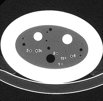
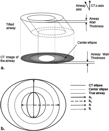
A lung phantom with six polycarbonate tubes embedded in foam was scanned, and the cross-sectional dimensions of the tubes were determined using the full width at half maximum, zero crossing, and phase congruency edge detection methods. Equations were derived using the reported wall intensity to correct for partial volume averaging. Corrections for the overestimation of the wall thickness due to the tilt of the tube with respect to the CT z-axis were also derived.

Results

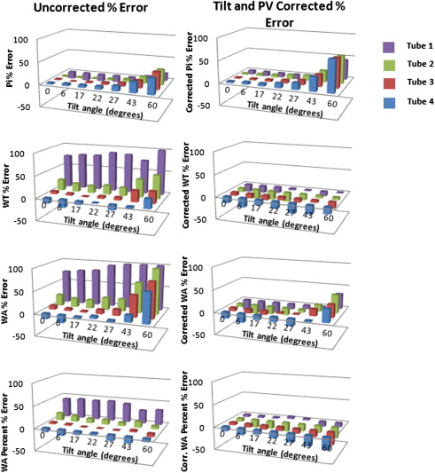
All three methods (full width at half maximum, zero crossing, and phase congruency) overestimated the wall thickness of the small polycarbonate tubes. It was verified that two sources of error were partial volume averaging and tilt that was introduced when the phantom was positioned with tube axes at an angle to the CT z-axis. The corrections were applied to the measured tube wall dimensions and substantially reduced the deviation of the CT measurements from the true values.

Conclusions

Correcting for partial volume effects and airway tilt greatly increases the accuracy of simulated airway wall measurements in transverse CT images.

Now that the size and luminal area of proximal airways can be measured in vivo using computed tomographic (CT) images, there is increasing interest in determining the relationship between airway dimensions and clinical indices of chronic obstructive pulmonary disease. CT studies of patients with a range of smoking histories have demonstrated associations between the severity of chronic obstructive pulmonary disease and airway characteristics . Because most of the resistance to airflow occurs in chronic obstructive pulmonary disease in the small airways , attention has turned to measuring small airways in CT images. However, technical limitations exist.

Although CT images of airways as small as 1.5 to 2.0 mm in diameter can be obtained and measured with reasonable accuracy , no airway segmentation method has yet emerged as a widely accepted standard. Most methods are either custom designed for the sole use of the developers or obtainable from commercial entities for licensing fees. Moreover, the commonly used full width at half maximum (FWHM) method of edge detection is known to overestimate wall thicknesses, especially for airways that are <2 mm in inner diameter (ID) .

Get Radiology Tree app to read full this article<

Materials and methods

Phantom

Get Radiology Tree app to read full this article<

Table 1

Calculated and Measured Airway Tube Cross-sectional Dimensions

Pi (mm) WT (mm) WA (mm 2 ) WA% Tube Tilt ID ∗ (mm) OD ∗ (mm) Reference Value † Mean SD Reference Value † Mean SD Reference Value † Mean SD Reference Value † 1t 30° 3.0 4.2 9.42 8.35 0.25 0.60 1.17 0.06 6.79 14.12 0.57 48.98 1 0° 3.0 4.2 9.42 7.95 0.06 0.60 1.05 0.01 6.79 11.82 0.12 48.98 2 0° 6.0 7.8 18.85 18.66 0.04 0.90 1.02 0.01 19.51 22.20 0.33 40.83 3t 30° 6.0 8.4 18.85 20.22 0.15 1.20 1.34 0.07 27.14 32.70 1.81 48.98 3 0° 6.0 8.4 18.85 19.19 0.04 1.20 1.11 0.00 27.14 25.27 0.07 48.98 4 0° 6.0 9.0 18.85 19.19 0.82 1.50 1.30 0.12 35.34 29.67 1.19 55.56

ID, inner diameter; OD, outer diameter; Pi, inner perimeter; SD, standard deviation; WA, wall area; WA%, wall area percentage; WT, wall thickness.

Measurements were made using the phase congruency method over seven contiguous 1 mm thick slices.

Get Radiology Tree app to read full this article<

CT Scanning

Get Radiology Tree app to read full this article<

Table 2

Measured Values of Pi and WT at Several FOVs

Measured Value, Phase Congruency Method Tube Reference Value (mm) FOV = 100 mm FOV = 150 mm FOV = 200 mm FOV = 350 mm Pi (mm) 1 9.42 8.36 8.37 8.28 7.97 2 18.85 18.44 18.33 18.33 18.39 4 18.85 19.22 19.48 19.46 19.39 WT (mm) 1 0.60 0.99 0.98 1.01 1.05 2 0.90 1.15 1.14 1.14 1.12 4 1.50 1.41 1.42 1.42 1.33 Reference WT (pixels) 1 3.13 2.05 1.54 0.88 2 4.69 3.07 2.30 1.32 4 7.82 5.12 3.84 2.19

FOV, field of view; Pi, inner perimeter; WT, wall thickness.

Get Radiology Tree app to read full this article<

Airway Analysis

Get Radiology Tree app to read full this article<

Measurement Correction Assumptions

Get Radiology Tree app to read full this article<

Partial Volume Correction

Get Radiology Tree app to read full this article<

WTm=WTw+WTl+WTp. WT

Get Radiology Tree app to read full this article<

I=I0e−μwWTwe−μlWTle−μpWTp, I

−

where μ w , μ l , and μ p are the linear attenuation of the tube, lumen, and parenchyma included in the pixel. Then, defining μ m as the linear attenuation of the pixel (equation 3a ) and converting to HU (equation 3b ) gives

I0e−μmWTm=I0e−μwWTwe−μlWTle−μpWTp I

−

and

HUmWTm=HUwWTw+HU1WT1+HUpWTp. HU

where HU w , HU l , and HU p are the attenuation of wall, lumen, and parenchyma in HU, and HU m is the mean attenuation of the airway wall. Because the wall thickness is determined by looking radially outward from the center of the airway, the true wall thickness WT w can be calculated from WT m .

Get Radiology Tree app to read full this article<

PVC=⎧⎩⎨⎪⎪⎪⎪HUm−HUl+HUp2HUw−HUl+HUp2HUm−HUlHUw−HUlID≥6pixelsID<6pixels PVC

{

−

≥

pixels

−

pixels

Get Radiology Tree app to read full this article<

WTw=PVC×WTm. WT

PVC

Get Radiology Tree app to read full this article<

WA=π(aobo−aibi) WA

(

−

)

and

WA%=100(1−aibiaobo). WA

100

(

−

)

Get Radiology Tree app to read full this article<

Tilt Correction

Get Radiology Tree app to read full this article<

Results

Partial Volume Correction

Get Radiology Tree app to read full this article<

Table 3

Measured and Partial Volume–corrected Dimensions of Nontilted Airway Tubes Using Each Segmentation Method (FWHM, ZC, and PC)

Measured Value, FOV = 350 mm Partial Volume–corrected Value Tube Reference Value ∗ FWHM ZC PC FWHM ZC PC Pi (mm) 1 9.42 7.72 8.29 7.97 7.74 8.30 8.02 2 18.85 18.1 18.61 18.39 19.02 19.34 19.25 3 18.85 18.41 19.03 19.13 18.05 19.35 19.18 4 18.85 18.88 19.65 19.39 19.15 19.61 19.41 WT (mm) 1 0.6 1.12 0.99 1.05 0.64 0.59 0.61 2 0.9 1.16 1.02 1.12 0.87 0.79 0.85 3 1.2 1.27 1.15 1.27 1.43 1.04 1.12 4 1.5 1.42 1.26 1.33 1.37 1.25 1.31 WA (mm 2 ) 1 6.79 12.56 11.26 11.79 6.33 5.63 6.19 2 19.51 25.14 22.15 24.45 18.71 17.10 18.39 3 27.14 28.52 26.07 29.46 32.31 23.52 25.57 4 35.34 33.24 29.61 31.28 32.18 29.48 30.71 WA% 1 48.98 72.51 67.11 69.83 57.19 50.66 55.01 2 40.83 48.98 44.43 47.5 39.39 36.49 38.42 3 48.98 51.08 47.45 50.84 55.49 44.12 46.62 4 55.56 53.75 49.02 51.07 52.45 49.08 50.60

FOV, field of view; FWHM, full width at half maximum; PC, phase congruency; Pi, inner perimeter; WA, wall area; WA%, wall area percentage; WT, wall thickness; ZC, zero crossing.

Get Radiology Tree app to read full this article<

Tilt Correction

Get Radiology Tree app to read full this article<

Table 4

Measured Tube 1 Wall Dimensions Compared to the Tilt-corrected Wall Dimensions

Angle (°) Pi m (Reference = 9.42 mm) Pi corr WT m (Reference = 0.6 mm) WT corr WA m (Reference = 6.79 mm 2 ) WA corr WA% m (Reference = 48.98%) WA% corr 0 7.97 8.59 1.05 0.85 11.79 9.62 69.83 62.11 6 7.86 8.50 1.08 0.88 12.09 9.87 70.95 63.20 17 8.01 8.57 1.08 0.90 12.29 10.32 70.49 63.89 22 8.16 8.48 1.13 1.03 13.20 12.15 71.17 68.12 27 8.58 8.81 1.12 1.05 13.50 12.73 69.57 67.52 43 10.03 10.81 1.05 0.92 14.15 12.67 63.38 59.44 60 10.97 13.56 1.31 1.05 19.97 18.44 65.22 62.46

corr, corrected value; m, measured value; Pi, inner perimeter; WA, wall area; WA%, wall area percentage; WT, wall thickness.

All measurements were made using the phase congruency method and a 350-mm field of view. References values were based on inner and outer diameters reported by manufacturer.

Get Radiology Tree app to read full this article<

Partial Volume and Tilt Correction

Get Radiology Tree app to read full this article<

Discussion

Get Radiology Tree app to read full this article<

Conclusions

Get Radiology Tree app to read full this article<

Acknowledgment

Get Radiology Tree app to read full this article<

Appendix

Partial Volume–Corrected Wall Dimensions

Get Radiology Tree app to read full this article<

I=I0e−(μmWTm), I

−

(

)

where μ m depends on the x-ray beam energy E and also on the materials that constitute the object. In general, the denser the material, the more the beam is attenuated as it travels through the material, so μ is larger for denser materials. If the object consists of three materials, lumen, wall, and parenchyma, with the beam traveling through them one at a time, the intensity is reduced as it travels through each material. If the beam has an intensity I p as it leaves the parenchyma and an intensity I w as it leaves the wall,

Ip=I0e−(μpWTp) I

−

(

)

and

Iw=Ipe−(μwWTw). I

−

(

)

Get Radiology Tree app to read full this article<

I=Iwe−(μlWTl) I

−

(

)

and

I=I0e−(μpWTp+μwWTw+μlWTl). I

−

(

)

Get Radiology Tree app to read full this article<

µmWTm=µpWTp+µwWTw+µlWTl. µ

Get Radiology Tree app to read full this article<

HU=1000×μ−μwaterμwater−μair HU

1000

−

water

−

air

as follows. Dividing both sides of equation A4 by (μ water − μ air ) gives

μmμwater−μairWTm=μpμwater−μairWTp+μwμwater−μairWTw+μlμwater−μairWTl. μ

water

−

air

water

−

air

water

−

air

water

−

air

Get Radiology Tree app to read full this article<

WTm=WTp+WTw+WTl, WT

so that

μwaterμwater−μairWTm=μwaterμwater−μair(WTp+WTw+WTl), μ

water

−

air

water

−

air

(

)

equation A6c can be subtracted from equation A6a :

μm−μwaterμwater−μairWTm=μp−μwaterμwater−μairWTp+μw−μwaterμwater−μairWTw+μl−μwaterμwater−μairWTl. μ

−

water

−

air

−

water

−

air

−

water

−

air

−

water

−

air

Get Radiology Tree app to read full this article<

HUmWTm=HUpWTp+HUwWTw+HUlWTl. HU

Get Radiology Tree app to read full this article<

HUmWTm=HUwWTw+HUpWTp+αHUlWTp. HU

Get Radiology Tree app to read full this article<

WTm=WTw+(1+α)WTp WT

(

)

and

WTp=WTm−WTw1+α. WT

−

Get Radiology Tree app to read full this article<

HUmWTm=HUwWTw+HUpWTm−WTw1+α+αHUlWTm−WTw1+α, HU

−

αHU

−

HUmWTm=HUwWTw+(HUp+αHUl)1+α(WTm−WTw), HU

(

αHU

)

(

−

)

and

(HUm−(HUp+αHUl)1+α)WTm=(HUw−(HUp+αHUl)1+α)WTw. (

−

(

αHU

)

(

−

(

αHU

)

Get Radiology Tree app to read full this article<

WTw=HUm−HUp+αHUl1+αHUw−HUp+αHUl1+αWTm WT

−

αHU

−

αHU

is the value of the true wall thickness in terms of the measured wall thickness WT m and the parameter α. It is possible to determine the best value of α empirically by calculating WT w with several values of α and using the value that results in the smallest percentage error of the corrected wall thickness WT w . For convenience, a PVC is defined as

PVC=HUm−HUp+αHUl1+αHUw−HUp+αHUl1+α, PVC

−

αHU

−

αHU

so that

WTw=(PVC)WTm. WT

(

PVC

)

Get Radiology Tree app to read full this article<

References

1. Berger P., Perot V., Desbarats P., et. al.: Airway wall thickness in cigarette smokers: quantitative thin-section CT assessment. Radiology 2005; 235: pp. 1055-1064.
2. Hasegawa M., Nasuhara Y., Onodera Y., et. al.: Airflow limitation and airway dimensions in chronic obstructive pulmonary disease. Am J Respir Crit Care Med 2006; 173: pp. 1309-1314.
3. Nakano Y., Muro S., Sakai H., et. al.: Computed tomographic measurements of airway dimensions and emphysema in smokers, correlation with lung function. Am J Respir Crit Care Med 2000; 162: pp. 1102-1108.
4. Orlandi I., Moroni C., Camiciottoli G., et. al.: Chronic obstructive pulmonary disease: thin-section CT measurement of airway wall thickness and lung attenuation. Radiology 2005; 234: pp. 604-610.
5. Macklem P.T., Mead J.: Resistance of central and peripheral airways measured by the retrograde catheter. J Appl Physiol 1967; 22: pp. 395-401.
6. Hogg J.C., Macklem P.T., Thurlbeck W.M.: Site and nature of airways obstruction in chronic obstructive lung disease. N Engl J Med 1968; 278: pp. 1355-1360.
7. King G., Müller N.L., Paré P.D.: Evaluation of airways in obstructive pulmonary disease using high-resolution computed tomography. Am J Respir Crit Care Med 1999; 159: pp. 998-1004.
8. Reinhardt J.M., D’Souza N.D., Hoffman E.A.: Accurate measurement of intra-thoracic airways. IEEE Trans Med Imaging 1997; 16: pp. 820-827.
9. Washko G.R., Dransfield M.T., Estépar R.S.J., et. al.: Airway wall attenuation: a biomarker of airway disease in subjects with COPD. J Appl Physiol 2009; 107: pp. 185-191.
10. Achenbach T., Weinheimer O., Dueber C., et. al.: Influence of pixel size on quantification of airway wall thickness in computed tomography. J Comput Assist Tomogr 2009; 33: pp. 725-730.
11. King G., Müller N.L., Paré P.D.: An analysis algorithm for measuring airway lumen and wall areas from high-resolution computed tomographic data. Am J Respir Crit Care Med 2000; 161: 574–480
12. Saba O.I., Hoffman E.A., Reinhardt J.M.: Maximizing quantitative accuracy of lung airway lumen and wall measures obtained from X-ray CT imaging. J Appl Physiol 2003; 95: pp. 1063-1075.
13. Estépar R.S.J., Washko G.R., Silverman E.K., et. al.: Accurate airway wall estimation using phase congruency.Larson R.Nielson M.Sporring J.MICCAI, LNCS 4191.2006.Springer-VerlagBerlin, Germany:pp. 125-134.
14. Estépar R.S.J., Washko G.R., Silverman E.K., et. al.: Airway Inspector: an open source application for lung morphometry. First Int Workshop Pulmon Image Process 2008; pp. 293-302.
15. Marr D., Hildreth E.: Theory of edge detection. Proc R Soc London B 1980; 208: pp. 187-217.
16. Kovesi P.: Phase congruency, a low level image invariant. Psychol Res 2000; 64: pp. 136-148.
17. Kovesi P. Edges are not just steps. Presented at: 5th Asian Conference on Computer Vision; 2002.
18. Amirav I., Kramer S., Grunstein M., et. al.: Assessment of methacholine-induced airway constriction with ultrafast high-resolution computed tomography. J Appl Physiol 1993; 75: pp. 2239-2250.
19. Kim W.J., Silverman E.K., Hoffman E., et. al.: CT metrics of airway disease and emphysema in severe COPD. Chest 2009; 136: pp. 396-404.
20. Wood S.A., Zerhouni E.A., Hoford J.D., et. al.: Measurement of three-dimensional lung tree structures by using computed tomography. J Appl Physiol 1995; 79: pp. 1687-1697.

Measuring Small Airways in Transverse CT Images

Rationale and Objectives

Materials and Methods

Results

Conclusions

Materials and methods

Phantom

CT Scanning

Airway Analysis

Measurement Correction Assumptions

Partial Volume Correction

Tilt Correction

Results

Partial Volume Correction

Tilt Correction

Partial Volume and Tilt Correction

Discussion

Conclusions

Acknowledgment

Appendix

Partial Volume–Corrected Wall Dimensions

References

Further Reading

A New Computerized Measurement Approach of Carotid Artery Stenosis on Tomographic Image Sequence

A Text-to-Speech Converter for Radiology Journal Articles

An Interactive Web-Based Tool for Detecting Verification (Work-up) Bias in Studies of the Efficacy of Diagnostic Imaging