Mixtures of Receiver Operating Characteristic Curves

Rationale and Objectives

Receiver operating characteristic (ROC) curves are ubiquitous in the analysis of imaging metrics as markers of both diagnosis and prognosis. While empirical estimation of ROC curves remains the most popular method, there are several reasons to consider smooth estimates based on a parametric model.

Materials and Methods

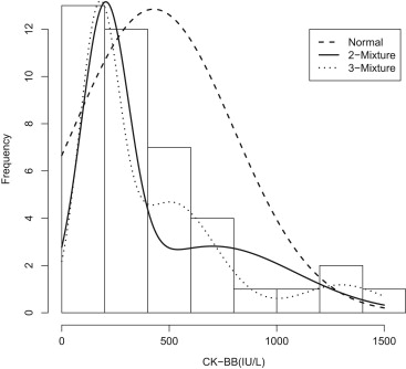
A mixture model is considered for modeling the distribution of the marker in the diseased population motivated by the biological observation that there is more heterogeneity in the diseased population than there is in the normal one. It is shown that this model results in an analytically tractable ROC curve which is itself a mixture of ROC curves.

Results

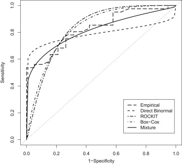
The use of creatine kinase–BB isoenzyme in diagnosis of severe head trauma is used as an example. ROC curves are fit using the direct binormal method, ROCKIT software, and the Box-Cox transformation as well as the proposed mixture model. The mixture model generates an ROC curve that is much closer to the empirical one than the other methods considered.

Conclusions

Mixtures of ROC curves can be helpful in fitting smooth ROC curves in datasets where the diseased population has higher variability than can be explained by a single distribution.

Receiver operating characteristic (ROC) curves have long become the standard way to describe the diagnostic accuracy of imaging methodologies. Initial applications of ROC curves in radiology focused on ordinal imaging metrics mostly based on reader evaluations . As quantitative imaging markers became more widely available, ROC curves were adapted in their evaluation . The use of ROC curves in evaluating predictive and prognostic models is quickly becoming standard as well . Several recent articles illustrate the recent methodological developments and the widening reach of ROC curves .

Given the depth and breadth of the applications of ROC curves in several fields it is no surprise that methodology for estimating ROC curves has proliferated. Many standard techniques are well-covered in several books that are largely or entirely devoted to the use of ROC curves . In addition software is available for major statistical packages like SAS (SAS Institue Inc, Cary, NC) , R (R Foundation, Vienna, Austria) , and Stata (StataCorp LP, College Station, TX) .

Get Radiology Tree app to read full this article<

Materials and methods

Mixture Models

Get Radiology Tree app to read full this article<

g(y)=λϕ1(y)+(1−λ)ϕ2(y) g

(

)

(

)

(

−

)

(

)

where λ is known as the mixing proportion and ϕ1 ϕ

1 and ϕ2 ϕ

2 are known as the component densities; both normal in this case, with possibly different means and variances (ie, ϕj ϕ

j has mean μj μ

j and standard deviation σj σ

j ). It is possible to represent a variety of probability distributions with this formulation due to the flexibility afforded by the component densities as well as the mixing proportion.

Get Radiology Tree app to read full this article<

g(y)=∑pj=1λjϕj(y) g

(

)

∑

(

)

where p is the number of components of the mixture. Estimation of p -component mixtures follow the same principles as estimation of two-component mixtures. In particular. it is common to use maximum likelihood to estimate the parameters of this mixture density .

Get Radiology Tree app to read full this article<

Mixture ROC Curves

Get Radiology Tree app to read full this article<

ROC(t)=G(G−10(t)) R

(

)

(

−

(

)

where 0 < t < 1 and the survivor function is 1 – the corresponding cumulative distribution:

G(x)=∫x∞g(y)dy G

(

)

∫

∞

(

)

with g(.) denoting the density function. If g(.) is a p -component mixture, then so is G(.):

G(x)=∑pj=1λjGj(x) G

(

)

∑

(

)

Get Radiology Tree app to read full this article<

ROC(p)(t)=∑pj=1λjGj(G−10(t)) ROC

(

)

(

)

∑

(

−

(

)

Get Radiology Tree app to read full this article<

aj=μj−μ0σj a

−

and

bj=σ0σj b

Get Radiology Tree app to read full this article<

Gj(G−10(t))=Φ(aj+bjΦ−1(t)) G

(

−

(

)

(

−

(

)

and the p -mixture ROC curve can be represented as

ROC(p)(t)=∑pj=1λjΦ(aj+bjΦ−1(t)) R

(

)

(

)

∑

(

−

(

)

Get Radiology Tree app to read full this article<

Summary Measures of the Mixture ROC Curve

Get Radiology Tree app to read full this article<

AUC=Φ(a1+b2√) A

(

)

Get Radiology Tree app to read full this article<

AUC(p)=∑pj=1λjAUCj A

(

)

∑

Get Radiology Tree app to read full this article<

AUC(p)=∑pj=1λjAUCj=∑pj=1λjΦ(aj1+b2j√) A

(

)

∑

(

)

Get Radiology Tree app to read full this article<

pAUC(p)=∑pj=1λjpAUCj p

(

)

∑

Get Radiology Tree app to read full this article<

ROC(p)(t)=∑pj=1λjGj(G−10(t))∣∣t=t0 R

(

)

(

)

∑

(

−

(

)

and when the threshold is c is given by

ROC(p)(t)=∑pj=1λjGj(G−10(t))∣∣t=G0(c) R

(

)

(

)

∑

(

−

(

)

(

)

Get Radiology Tree app to read full this article<

Results

Get Radiology Tree app to read full this article<

Table 1

Estimates of the Moments of the Diseased Distribution

Mean Standard Deviation Skewness Kurtosis Empirical 427 373 1.42 1.44 Binormal 427 373 0 0 2-Mixture 427 368 1.07 0.60 3-Mixture 427 368 1.41 1.50

Get Radiology Tree app to read full this article<

Table 2

Estimates of the Area Under the Curve (AUC) and the Sensitivity at Three Different Operating Points for the Five Receiver Operating Characteristic Curves Plotted in Figure 2

AUC Sensitivity (Specificity = 0.60) Sensitivity (Specificity = 0.75) Sensitivity (Specificity = 0.90) Empirical 0.828 0.818 0.683 0.561 Direct binormal 0.790 0.777 0.745 0.693 ROCKIT 0.831 0.908 0.750 0.382 Box-Cox 0.831 0.887 0.742 0.427 Mixture 0.815 0.803 0.717 0.598

Get Radiology Tree app to read full this article<

Discussion

Get Radiology Tree app to read full this article<

Appendices

Appendix A

Get Radiology Tree app to read full this article<

Mean=μ=∑pj=1λjμjVariance=σ2=∑pj=1λj(σ2j−μ2j)−μ2Skewness=1σ3∑pj=1λj(μj−μ)[3σ2j+(μj−μ)2]Kurtosis=1σ4∑pj=1λj[3σ4j+6σ2j(μj−μ)2+(μj−μ)4]−3 Mean

∑

Variance

∑

(

−

)

−

Skewness

∑

(

−

)

[

(

−

)

]

Kurtosis

∑

[

(

−

)

(

−

)

]

−

Get Radiology Tree app to read full this article<

Appendix B

Get Radiology Tree app to read full this article<

normalmixEM(poor,lambda=0.5,mu=c(200,700),sigma=c(10,50)) n

(

poor

lambda

0.5

(

200

700

)

sigma

(

)

Get Radiology Tree app to read full this article<

boot.comp(poor,mix.type=”normalmix”) b

(

”

)

Get Radiology Tree app to read full this article<

References

1. Goodenough D.J., Rossmann K., Lusted L.B.: Radiographic applications of receiver operating characteristic (ROC) curves. Radiology 1974; 110: pp. 89-95.
2. Starr S.J., Metz C.E., Lusted L.B., et. al.: Visual detection and localization of radiographic images. Radiology 1975; 116: pp. 533-538.
3. Metz C.E.: ROC methodology in radiologic imaging. Investigative radiology 1986; 21: pp. 720.
4. Gatsonis C., Begg C., Wieand S.: Advances in statistical methods for diagnostic radiology: a symposium. Acad Radiol 1995; 2: pp. S1-S84.
5. Wong R., Lin D., Schöder H., et. al.: Diagnostic and prognostic value of [18F] fluorodeoxyglucose positron emission tomography for recurrent head and neck squamous cell carcinoma. J Clin Oncol 2002; 20: pp. 4199-4208.
6. Yuan Y., Giger M.L., Li H., et. al.: Multimodality computer-aided breast cancer diagnosis with FFDM and DCE-MRI. Acad Radiol 2010; 17: pp. 1158.
7. Tsushima Y., Takano A., Taketomi-Takahashi A., et. al.: Body diffusion-weighted MR imaging using high b -value for malignant tumor screening: usefulness and necessity of referring to T2-Weighted images and creating fusion images. Acad Radiol 2007; 14: pp. 643-650.
8. Güttler A.: Using a bootstrap approach to rate the raters. Fin Markets Portfolio Manage 2005; 19: pp. 277-295.
9. Mailier P., Jollife I., Stephenson D.: Quality of weather forecasts. Review and recommendations R Meteorol Soc 2006; pp. 1-89. Available at http://empslocal.ex.ac.uk/people/staff/dbs202/publications/booksreports/mailier.pdf
10. Steyerberg E.W., Vickers A.J., Cook N.R., et. al.: Assessing the performance of prediction models: a framework for traditional and novel measures. Epidemiology 2010; 21: pp. 128.
11. Alemayehu D., Zou K.H.: Applications of ROC analysis in medical research: recent developments and future directions. Acad Radiol 2012; 19: pp. 1457-1464.
12. Skaron A., Li K., Zhou X.H.: Statistical methods for MRMC ROC studies. Acad Radiol 2012; 19: pp. 1499-1507.
13. Obuchowski N.A., Gallas B.D., Hillis S.L.: Multi-reader ROC studies with split-plot designs: a comparison of statistical methods. Acad Radiol 2012; 19: pp. 1508-1517.
14. Gönen M.: Analyzing receiver operating characteristic curves with SAS.2007.SAS InstituteCary, NC
15. Krzanowski W.J.: ROC curves for continuous data.2009.Chapman & Hall/CRCBoca Raton, FL
16. Pepe M.S.: The statistical evaluation of medical tests for classification and prediction.2004.Oxford University PressNew York, NY
17. Zhou X.H., McClish D.K., Obuchowski N.A.: Statistical methods in diagnostic medicine.2009.Wiley-InterscienceHoboken, NJ
18. Robin X., Turck N., Hainard A., et. al.: pROC: an open-source package for R and S+ to analyze and compare ROC curves. BMC Bioinform 2011; 12: pp. 77.
19. Hillis S.L.: Simulation of unequal-variance binormal multireader ROC decision data: an extension of the Roe and Metz simulation model. Acad Radiol 2012; 19: pp. 1518-1528.
20. Zou K.H., Tempany C.M., Fielding J.R., et. al.: Original smooth receiver operating characteristic curve estimation from continuous data: statistical methods for analyzing the predictive value of spiral CT of ureteral stones. Acad Radiol 1998; 5: pp. 680-687.
21. Zou K.H., Hall W.: Two transformation models for estimating an ROC curve derived from continuous data. J Appl Stat 2000; 27: pp. 621-631.
22. Metz C.E., Herman B.A., Shen J.H.: Maximum likelihood estimation of receiver operating characteristic (ROC) curves from continuously-distributed data. Stat Med 1998; 17: pp. 1033-1053.
23. Hans P., Albert A., Born J., et. al.: Derivation of a bioclinical prognostic index in severe head injury. Intens Care Med 1985; 11: pp. 186-191.
24. McLachlan G., Peel D.: Finite mixture models.2000.Wiley-InterscienceNew York, NY
25. McLachlan G.J., Krishnan T.: The EM algorithm and extensions.2007.Wiley-InterscienceNew York, NY
26. McClish D.K.: Analyzing a portion of the ROC curve. Med Decis Making 1989; 9: pp. 190-195.
27. Hillis S.L., Metz C.E.: An analytic expression for the binormal partial area under the ROC curve. Acad Radiol 2012; 19: pp. 1491-1498.
28. McLachlan G.J.: On bootstrapping the likelihood ratio test stastistic for the number of components in a normal mixture. Appl Stat 1987; 36: pp. 318-324.
29. Metz C.: ROCKIT 0.9 B. Beta version.1998.Department of Radiology, University of Chicago
30. Goddard M.J., Hinberg I.: Receiver operator characteristic (ROC) curves and non-normal data: an empirical study. Stat Med 1990; 9: pp. 325-337.
31. Hanley J.A.: The robustness of the “binormal” assumptions used in fitting ROC curves. Med Decis Making 1988; 8: pp. 197-203.
32. Metz C.E., Kronman H.B.: Statistical significance tests for binormal ROC curves. J Math Psychol 1980; 22: pp. 218-243.
33. Metz C.E., Pan X.: “Proper” binormal ROC curves: theory and maximum-likelihood estimation. J Math Psychol 1999; 43: pp. 1-33.
34. Pesce L.L., Metz C.E., Berbaum K.S.: On the convexity of ROC curves estimated from radiological test results. Acad Radiol 2010; 17: pp. 960-968. e4
35. Lloyd C.J.: Using smoothed receiver operating characteristic curves to summarize and compare diagnostic systems. J Am Stat Assoc 1998; 93: pp. 1356-1364.
36. Cai T.: Semi-parametric ROC regression analysis with placement values. Biostatistics 2004; 5: pp. 45-60.
37. Pepe M.S.: An interpretation for the ROC curve and inference using GLM procedures. Biometrics 2000; 56: pp. 352-359.
38. Zou K.H., Hall W.J., Shapiro D.E.: Smooth non-parametric receiver operating characteristic (ROC) curves for continuous diagnostic tests. Stat Med 1997; 16: pp. 2143-2156.
39. Benaglia T., Chauveau D., Hunter D.R., et. al.: mixtools: An R package for analyzing finite mixture models. J Stat Software 2009; 32: pp. 1-29.
40. Frühwirth-Schnatter S.: Finite mixture and Markov switching models.2006.Springer Science + Business Media, LLCNew York, NY

Mixtures of Receiver Operating Characteristic Curves

Rationale and Objectives

Materials and Methods

Results

Conclusions

Materials and methods

Mixture Models

Mixture ROC Curves

Summary Measures of the Mixture ROC Curve

Results

Discussion

Appendices

Appendix A

Appendix B

References

Further Reading

A Brief History of Free-Response Receiver Operating Characteristic Paradigm Data Analysis

An Additive Selection of Markers to Improve Diagnostic Accuracy Based on a Discriminatory Measure

An Examination of Data Confidentiality and Disclosure Issues Related to Publication of Empirical ROC Curves