
Rationale and Objectives
Magnetic resonance imaging (MRI)-based texture analysis has been shown to be effective in classifying multiple sclerosis lesions. Regarding the clinical use of texture analysis in multiple sclerosis, our intention was to show which parts of the analysis are sensitive to slight changes in textural data acquisition and which steps tolerate interference.
Materials and Methods
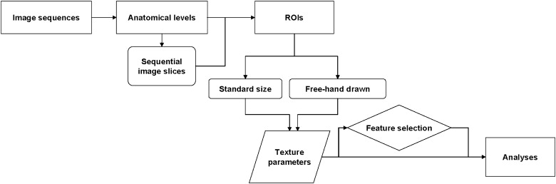
The MRI datasets of 38 multiple sclerosis patients were used in this study. Three imaging sequences were compared in quantitative analyses, including a comparison of anatomical levels of interest, variance between sequential slices and two methods of region of interest drawing. We focused on the classification of white matter and multiple sclerosis lesions in determining the discriminatory power of textural parameters. Analyses were run with MaZda software for texture analysis, and statistical tests were performed for raw parameters.
Results
MRI texture analysis based on statistical, autoregressive-model and wavelet-derived texture parameters provided an excellent distinction between the image regions corresponding to multiple sclerosis plaques and white matter or normal-appearing white matter with high accuracy (nonlinear discriminant analysis 96%–100%). There were no significant differences in the classification results between imaging sequences or between anatomical levels. Standardized regions of interest were tolerant of changes within an anatomical level when intra-tissue variance was tested.
Conclusion
The MRI texture analysis protocol with fixed imaging sequence and anatomical levels of interest shows promise as a robust quantitative clinical means for evaluating multiple sclerosis lesions.
Multiple sclerosis (MS) is the most common autoimmune disease of the central nervous system, with complex pathophysiology, including inflammation, demyelination, axonal degeneration, and neuronal loss. According to recent pathological evidence, these processes are not similarly represented in different patients, but may predominate selectively in individual patients, leading to heterogeneity in the expression of disease phenotypes. This diverse representation of different pathologies is also reflected in disease prognosis and response to therapies.
Diagnostic evaluation of MS with conventional magnetic resonance imaging (MRI) is generally based on the McDonald criteria . The development of modern imaging techniques for the early detection of brain inflammation and the characterization of tissue-specific injury is an important objective in MS research. The development of new imaging techniques is targeted especially at the identification of high-risk individuals in the early phase of MS disease and at the improved monitoring of disease activity. A better understanding of disease pathogenesis is also the basis for the further development of new and more effective therapies.
Get Radiology Tree app to read full this article<
Get Radiology Tree app to read full this article<
Get Radiology Tree app to read full this article<
Get Radiology Tree app to read full this article<
Materials and Methods
Patients
Get Radiology Tree app to read full this article<
MRI Acquisition
Get Radiology Tree app to read full this article<
Texture Analysis
Get Radiology Tree app to read full this article<
Get Radiology Tree app to read full this article<
Get Radiology Tree app to read full this article<
Get Radiology Tree app to read full this article<
Get Radiology Tree app to read full this article<
Table 1
Tissues Used as ROIs and Sizes of ROIs in Pixels
ROI Size White matter 10 × 10 Normal-appearing white matter 10 × 10 Cerebrospinal fluid 10 × 10 Normal-appearing gray matter apart lesion 6 × 6 Normal-appearing gray matter near lesion 6 × 6 Nucleus caudatus 10 × 10 Nucleus lentiformis 10 × 10 MS plaque, freehand ROI Varying MS plaque, standard size ROI 10 × 10
MS = multiple sclerosis; ROI = region of interest.
Get Radiology Tree app to read full this article<
Get Radiology Tree app to read full this article<
Get Radiology Tree app to read full this article<
Get Radiology Tree app to read full this article<
Get Radiology Tree app to read full this article<
Table 2
Tissue Pairs Used in the Classification of Tissues
Tissue pairs used in classification White matter/MS plaque, freehand ROI White matter/MS plaque, 10 × 10 ROI White matter/normal-appearing white matter Normal appearing white matter/MS plaque, freehand ROI Normal appearing white matter/MS plaque, 10 × 10 ROI Nucleus caudatus/nucleus lentiformis
MS = multiple sclerosis; ROI = region of interest.
Get Radiology Tree app to read full this article<
Get Radiology Tree app to read full this article<
Table 3
List of 25 Texture Analysis Parameters used in Manual Feature Selection
Parameters used in Manual Feature Selection Parameter Group Parameter Name Cooccurrence matrix Contrast S(0,1) Cooccurrence matrix Contrast S(1,0) Cooccurrence matrix Contrast S(1,1) Cooccurrence matrix Contrast S(1,-1) Cooccurrence matrix Difference variance S(0,1) Cooccurrence matrix Difference variance S(1,0) Cooccurrence matrix Difference variance S(1,1) Cooccurrence matrix Difference variance S(1,-1) Cooccurrence matrix Sum of squares S(0,1) Cooccurrence matrix Sum of squares S(1,0) Cooccurrence matrix Sum of squares S(1,1) Cooccurrence matrix Sum of squares S(1,-1) Cooccurrence matrix Sum variance S(0,1) Cooccurrence matrix Sum variance S(1,0) Cooccurrence matrix Sum variance S(1,1) Cooccurrence matrix Sum variance S(1,-1) Run length matrix Gray level nonuniformity, 135° Run length matrix Gray level nonuniformity, 45° Run length matrix Gray level nonuniformity, 0° Run length matrix Gray level nonuniformity, 90° Gradient Mean absolute gradient Gradient Variance of absolute gradient Autoregressive model Standard deviation Wavelet Energy, subband 1, HL Wavelet Energy, subband 2, HL
Get Radiology Tree app to read full this article<
Get Radiology Tree app to read full this article<
Results
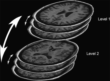
Intra-tissue Difference in Sequential Image Slices and between Anatomical Levels
Get Radiology Tree app to read full this article<
Table 4
Intra-tissue Differences between Anatomical Levels Calculated for Three Imaging Sequences
Imaging Sequence T1 MPR T1 MPR+C T2 TIRM_n_ % of Total_n_ % of Total_n_ % of Total WM 9 3% 18 6% 35 12% NAWM 3 1% 8 3% 7 2% CSF 20 7% 28 10% 20 7% NAGM apart lesion 18 6% 21 7% 26 9% NAGM near lesion 7 2% 9 3% 10 4% MS plaque, freehand ROI 46 16% 94 34% 85 30% MS plaque, 10 × 10 ROI 13 5% 22 8% 13 5%
MPR = magnetization prepared gradient echo sequence; MPR+C = T1 MPR with contrast agent; WM = white matter; NAWM = normal-appearing white matter; CSF = cerebrospinal fluid NAGM = normal-appearing gray matter; MS = multiple sclerosis; ROI = region of interest.
The number and percentage of parameters having statistically significant difference in the Wilcoxon test ( P < .05) are given in columns; the total number of parameters was 280. The total number of patients was 38.
Get Radiology Tree app to read full this article<
Get Radiology Tree app to read full this article<
Table 5
Intra-tissue Differences between Three Sequential Image Slices Calculated for T1-weighted Imaging Sequences T1 MPR and T1 MPR+C on Both Anatomical Levels with the Friedman Test
Imaging Sequence T1 MPR T1 MPR+C Imaging Level 1 2 1 2n % of Total_n_ % of Total_n_ % of Total_n_ % of Total WM 14 5% 20 7% 11 4% 15 5% NAWM 18 7% 13 5% 26 9% 12 4% CSF 3 1% 18 6% 17 6% 13 5% NAGM apart lesion 22 8% 18 6% 18 6% 18 6% NAGM near lesion 26 9% 26 9% 36 13% 21 8% Nucleus caudatus 24 9% 18 6% Nucleus lentiformis 11 4% 6 2% MS plaque, freehand ROI 14 5% 38 14% 36 13% 15 5% MS plaque, 10 × 10 ROI 17 6% 14 5% 20 7% 15 5%
MPR = magnetization prepared gradient echo sequence; MPR+C = T1 MPR with contrast agent; WM = white matter; NAWM = normal-appearing white matter; CSF = cerebrospinal fluid; NAGM = normal-appearing gray matter; MS = multiple sclerosis; ROI = region of interest.
Nucleus caudatus and nucleus lentiformis were visible only in level 2 and were thus left out of the analyses of level 1. The number and percentage of parameters having statistically significant differences ( P < .05) are given in columns. The total number of texture parameters was 280. The total number of patients was 23.
Get Radiology Tree app to read full this article<
Classification of Tissues
Get Radiology Tree app to read full this article<
Get Radiology Tree app to read full this article<
Tables 6a–c
Rate of Correct Classification of Tissue Pairs Independently Calculated for the Three Imaging Sequences T1 MPR (6a), T1 MPR+C (6b), and T2 TIRM (6c)
Table 6a T1 MPR Imaging Level Level 1 Level 2 Feature Selection F P M F P M WM vs. MS freehand ROI PCA 94% (72/76) 98% (75/76) 85% (65/76) 90% (69/76) 97% (74/76) 85% (65/76) NDA 100% (76/76) 100% (76/76) 100% (76/76) 98% (75/76) 100% (76/76) 98% (75/76) WM vs. MS 10 × 10 ROI PCA 94% (72/76) 96% (73/76) 78% (60/76) 81% (61/75) 94% (71/75) 81% (61/75) NDA 100% (76/76) 100% (76/76) 98% (75/76) 97% (73/75) 100% (75/75) 98% (74/75) NAWM vs. MS freehand ROI PCA 92% (70/76) 98% (75/76) 86% (66/76) 98% (75/76) 97% (74/76) 85% (65/76) NDA 100% (76/76) 100% (76/76) 100% (76/76) 100% (76/76) 100% (76/76) 100% (76/76) NAWM vs. MS 10 × 10 ROI PCA 90% (69/76) 90% (69/76) 81% (62/76) 93% (70/75) 97% (73/75) 85% (64/75) NDA 98% (75/76) 98% (75/76) 98% (75/76) 100% (75/75) 100% (75/75) 97% (73/75)
Table 6b T1 MPR+C Imaging Level Level 1 Level 2 Feature Selection F P M F P M WM vs. MS freehand ROI PCA 97% (73/75) 100% (75/75) 93% (70/75) 96% (73/76) 96% (73/76) 93% (71/76) NDA 100% (75/75) 100% (75/75) 100% (75/75) 100% (76/76) 100% (76/76) 98% (75/76) WM vs. MS 10 × 10 ROI PCA 92% (70/76) 94% (72/76) 82% (63/76) 96% (73/76) 97% (74/76) 77% (59/76) NDA 100% (76/76) 100% (76/76) 96% (73/76) 100% (76/76) 100% (76/76) 98% (75/76) NAWM vs. MS freehand ROI PCA 93% (70/75) 98% (74/75) 90% (68/75) 90% (69/76) 96% (73/76) 88% (67/76) NDA 96% (72/75) 100% (75/75) 100% (75/75) 98% (75/76) 97% (74/76) 98% (75/76) NAWM vs. MS 10 × 10 ROI PCA 94% (72/76) 92% (70/76) 81% (62/76) 100% (76/76) 98% (75/76) 82% (63/76) NDA 100% (76/76) 100% (76/76) 96% (73/76) 100% (76/76) 100% (76/76) 98% (75/76)
Table 6c T2 TIRM Imaging Level Level 1 Level 2 Feature Selection F P M F P M WM vs. MS freehand ROI PCA 100% (76/76) 100% (76/76) 89% (68/76) 98% (74/75) 100% (75/75) 96% (72/75) NDA 100% (76/76) 100% (76/76) 100% (76/76) 100% (75/75) 100% (75/75) 100% (75/75) WM vs. MS 10 × 10 ROI PCA 85% (65/76) 86% (66/76) 80% (61/76) 88% (66/75) 97% (73/75) 86% (65/75) NDA 97% (74/76) 98% (75/76) 96% (73/76) 97% (73/75) 100% (75/75) 98% (74/75) NAWM vs. MS freehand ROI PCA 98% (75/76) 100% (76/76) 93% (71/76) 100% (76/76) 100% (76/76) 89% (68/76) NDA 100% (76/76) 100% (76/76) 100% (76/76) 100% (76/76) 100% (76/76) 100% (76/76) NAWM vs. MS 10 × 10 ROI PCA 77% (59/76) 81% (81/76) 68% (52/76) 86% (66/76) 89% (68/76) 69% (53/76) NDA 96% (73/76) 96% (73/76) 98% (75/76) 97% (74/76) 98% (75/76) 98% (75/76)
Results are presented for two anatomical imaging levels: corona radiata and centrum semiovale and basal ganglia, for three feature reduction methods: Fisher (F), POE+ACC (P), and manual (M). Classifications were based on 1-NN for features of principal component analysis (PCA) and on ANN for nonlinear discriminant analysis (NDA) features. Data are percentages of correct classification. Data in parentheses are the number of region of interest (ROI) samples correctly classified and the total number of ROI samples in the analysis in question used to calculate percentages. The total number of patients was 38.
MPR = magnetization prepared gradient echo sequence; MPR+C = T1 MPR with contrast agent; WM = white matter; NAWM = normal-appearing white matter; CSF = cerebrospinal fluid NAGM = normal-appearing gray matter; MS = multiple sclerosis; ROI = region of interest.
Get Radiology Tree app to read full this article<
Get Radiology Tree app to read full this article<
Tables 7 a–c
The 10 Best Texture Parameters for White Matter and MS Classification Given Individually for Imaging Sequences T1 MPR (7a), T1 MPR+C (7b), and T2 TIRM (7c)
Table 7a T1 MPR Tissues WM NAWM MS, Freehand ROI MS, 10 × 10 ROI Imaging Level 1 2 1 2 1 2 1 2 Parameter Group, Name Md Md Md Md Md Md Md Md Autoregressive model Standard deviation 0.42 0.40 0.40 0.41 0.22 0.23 0.26 0.25 Histogram MinNorm 293 299 304 295 158 158 183 177 Histogram Variance 176 185 203 192 1102 1209 819 754 Gradient Mean absolute gradient 1088 1095 1091 1082 732 781 887 813 Cooccurrence matrix Contrast S(1,0) 988 932 877 860 410 448 588 529 Wavelet Energy, subband 2, LL 17,629 17,369 17,683 17,087 29,582 26,829 27,055 23,209 Co-occurrence matrix Sum entropy S(3,0) 1.65 1.62 1.66 1.64 2.17 2.06 1.73 1.75 Co-occurrence matrix Contrast S(0,1) 945 874 929 940 409 419 541 479 Co-occurrence matrix Sum entropy S(2,0) 1.70 1.71 1.72 1.72 2.22 2.11 1.79 1.80 Co-occurrence matrix Contrast S(2,0) 31,110 2840 2813 2618 1263 1448 1936 1595
Table 7b T1 MPR+C Tissues WM NAWM MS, Freehand ROI MS, 10 × 10 ROI Imaging Level 1 2 1 2 1 2 1 2 Parameter Group, Name Md Md Md Md Md Md Md Md Histogram MinNorm 297 299 310 295 162 162 167 170 Autoregressive model Standard deviation 0.43 0.39 0.40 0.39 0.24 0.21 0.27 0.21 Gradient Mean absolute gradient 1144 1109 1073 1075 772 775 895 835 Histogram Variance 183 179 185 184 1231 1422 730 749 Run length matrix Gray level nonuniformity, 90° 2.88 2.94 2.89 2.95 5.11 3.58 2.00 1.94 Wavelet Energy, subband 2, LL 17,076 16,812 18,352 18,651 27,477 27,614 25,828 24,621 Co-occurrence matrix Sum average S(1,1) 255 254 254 254 246 246 245 245 Co-occurrence matrix Sum entropy S(2,2) 1.63 1.64 1.64 1.63 2.22 2.09 1.71 1.71 Co-occurrence matrix Sum entropy S(1,0) 1.77 1.76 1.78 1.77 2.29 2.18 1.84 1.85 Run length matrix Gray level nonuniformity, 45° 2.85 3.00 2.85 2.93 5.14 3.55 2.04 2.06
Table 7c T2 TIRM Tissues WM NAWM MS, Freehand ROI MS, 10 × 10 ROI Imaging Level 1 2 1 2 1 2 1 2 Parameter Group, Name Md Md Md Md Md Md Md Md Co-occurrence matrix Sum average S(1,0) 254 254 253 254 263 265 261 262 Co-occurrence matrix Sum average S(1,1) 254 255 253 252 265 266 268 268 Autoregressive model Standard deviation 0.41 0.42 0.38 0.34 0.15 0.18 0.23 0.19 Co-occurrence matrix Sum average S(1,-1) 254 255 253 253 265 267 266 268 Histogram Variance 165 162 193 221 2507 2073 906 1164 Co-occurrence matrix Sum average S(2,0) 253 255 254 254 268 269 264 267 Run length matrix Gray level nonuniformity, 135° 2.94 3.00 2.84 2.84 5.67 4.20 1.89 1.92 Co-occurrence matrix Sum average S(0,2) 253 256 254 253 269 267 264 263 Co-occurrence matrix Sum average S(0,1) 254 255 254 253 264 263 261 260 Co-occurrence matrix Contrast S(1,-1) 1307 1532 1275 1283 439 612 957 777
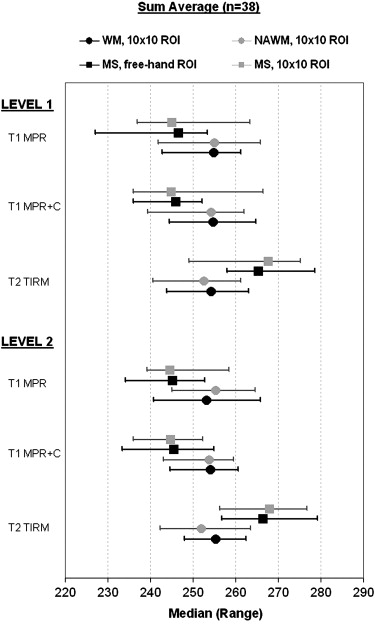
Texture feature distribution median values (Md) are given in columns for white matter (WM), normal-appearing white matter (NAWM), MS 10 × 10 and freehand regions of interest (ROIs). Statistical differences between the tissue pairs WM vs. MS freehand ROI, WM vs. MS 10 × 10 ROI, NAWM vs. MS freehand ROI, and NAWM vs. MS 10 × 10 ROI for imaging levels 1 and 2 was calculated with the Wilcoxon signed rank test. The results were uniform and are given in P values. Statistical differences between tissue pairs was highly significant ( P < .0001) in all comparisons except those mentioned in the table footnotes. The total number of patients was 38.
MPR = magnetization prepared gradient echo sequence; MPR+C = T1 MPR with contrast agent; WM = white matter; NAWM = normal-appearing white matter; CSF = cerebrospinal fluid NAGM = normal-appearing gray matter; MS = multiple sclerosis; ROI = region of interest.
Table 7b
1) Gray level nonuniformity, 90°: WM vs. MS freehand ROI, level 2: P = .0140; NAWM vs. MS freehand ROI; level 2: P = .0411.
2) Gray level nonuniformity, 45°: WM vs. MS freehand ROI, level 2: P = .0150; NAWM vs. MS freehand ROI; level 2: P = .0326.
Table 7c
1) Gray level nonuniformity, 135°: WM vs. MS freehand ROI, level 2: P =.0090.
2) Contrast S(1,-1): NAWM vs. MS 10 × 10 ROI, level 1: P = .0032.
Get Radiology Tree app to read full this article<
Discussion
Get Radiology Tree app to read full this article<
Get Radiology Tree app to read full this article<
Get Radiology Tree app to read full this article<
Get Radiology Tree app to read full this article<
Get Radiology Tree app to read full this article<
Get Radiology Tree app to read full this article<
Get Radiology Tree app to read full this article<
Get Radiology Tree app to read full this article<
Get Radiology Tree app to read full this article<
Get Radiology Tree app to read full this article<
Acknowledgment
Get Radiology Tree app to read full this article<
References
1. McDonald W.I., Compston A., Edan G., et. al.: Recommended diagnostic criteria for multiple sclerosis: guidelines from the international panel on the diagnosis of multiple sclerosis. Ann Neurol 2001; 50: pp. 121-127.
2. Polman C.H., Reingold S.C., Edan G., et. al.: Diagnostic criteria for multiple sclerosis: 2005 revisions to the “McDonald criteria.”. Ann Neurol 2005; 58: pp. 840-846.
3. Rovira À, León A.: MR in the diagnosis and monitoring of multiple sclerosis: an overview. Eur J Radiol 2008; 67: pp. 409-414.
4. Bakshi R., Thompson A.J., Rocca M.A., et. al.: MRI in multiple sclerosis: current status and future prospects. Lancet Neurol 2008; 7: pp. 615-625.
5. Bonilha L., Kobayashi E., Castellano G., et. al.: Texture analysis of hippocampal sclerosis. Epilepsia 2003; 44: pp. 1546-1550.
6. Bernasconi A., Antel S.B., Collins D.L., et. al.: Texture analysis and morphological processing of magnetic resonance imaging assist detection of focal cortical dysplasia in extra-temporal partial epilepsy. Ann Neurol 2001; 49: pp. 770-775.
7. Antel S.B., Collins D.L., Bernasconi N., et. al.: Automated detection of focal cortical dysplasia lesions using computational models of their MRI characteristics and texture analysis. NeuroImage 2003; 19: pp. 1748-1759.
8. Sankar T., Bernasconi N., Kim H., et. al.: Temporal lobe epilepsy: differential pattern of damage in temporopolar cortex and white matter. Hum Brain Mapp 2008; 29: pp. 931-944.
9. Mathias J.M., Tofts P.S., Losseff N.A.: Texture analysis of spinal cord pathology in multiple sclerosis. Magn Reson Med 1999; 42: pp. 929-935.
10. Yu O., Mauss Y., Zollner G., et. al.: Distinct patterns of active and non-active plaques using texture analysis on brain NMR images in multiple sclerosis patients: preliminary results. Magn Reson Imaging 1999; 17: pp. 1261-1267.
11. Theocharakis P., Glueer C., Kostopoulos S., et. al.: Pattern recognition system for the discrimination of multiple sclerosis from cerebral microangiopathy lesions based on texture analysis of magnetic resonance images. Magn Reson Imaging 2009; 27: pp. 417-422.
12. Loizou C.P., Pattichis C.S., Seimenis I., et. al.: Quantitative analysis of brain white matter lesions in multiple sclerosis subjects: preliminary findings. 2008; pp. 58-61.
13. Zhang J., Tong L., Wang L., et. al.: Texture analysis of multiple sclerosis: a comparative study. Magn Reson Imaging 2008; 26: pp. 1160-1166.
14. Herlidou-Meme S., Constans J.M., Carsin B., et. al.: MRI texture analysis on texture test objects, normal brain and intracranial tumors. Magn Reson Imaging 2003; 21: pp. 989-993.
15. Mahmoud-Ghoneim D., Toussaint G., Constans J., et. al.: Three dimensional texture analysis in MRI: a preliminary evaluation in gliomas. Magn Reson Imaging 2003; 21: pp. 983-987.
16. Georgiadis P., Cavouras D., Kalatzis I., et. al.: Enhancing the discrimination accuracy between metastases, gliomas and meningiomas on brain MRI by volumetric textural features and ensemble pattern recognition methods. Magn Reson Imaging 2009; 27: pp. 120-130.
17. Yu O., Parizel N., Pain L., et. al.: Texture analysis of brain MRI evidences the amygdala activation by nociceptive stimuli under deep anesthesia in the propofol–formalin rat model. Magn Reson Imaging 2007; 25: pp. 144-146.
18. Freeborough P.A., Fox N.C.: MR image texture analysis applied to the diagnosis and tracking of Alzheimer’s disease. IEEE Trans Med Imaging 1998; 17: pp. 475-479.
19. Torabi M.: Discrimination between Alzheimer’s disease and control group in MR-images based on texture analysis using artificial neural network. International Conference on Biomedical and Pharmaceutical Engineering (ICBPE) 2006; pp. 79-83.
20. Boniatis I., Panayiotakis G., Klironomos G., et. al.: Texture analysis of spinal cord signal in pre- and post-operative T2-weighted magnetic resonance images of patients with cervical spondylotic myelopathy. IEEE International Workshop on Imaging Systems and Techniques (IST) 2008; pp. 353-356.
21. Mayerhoefer M.E., Breitenseher M., Amann G., et. al.: Are signal intensity and homogeneity useful parameters for distinguishing between benign and malignant soft tissue masses on MR images? Objective evaluation by means of texture analysis. Magn Reson Imaging 2008; 26: pp. 1316-1322.
22. Szczypinski P.M., Strzelecki M., Materka A.: Mazda—a software for texture analysis. International Symposium on Information Technology Convergence (ISITC) 2007; pp. 245-249.
23. Szczypiński P.M., Strzelecki M., Materka A., et. al.: MaZda—A software package for image texture analysis. Comput Methods Programs Biomed 2009; 94: pp. 66-76.
24. Hajek M., Dezortova M., Materka A., et. al.: Texture analysis for magnetic resonance imaging.2006.Czech Republic: Med4publishing s.r.oPrague
25. Materka A, Strzelecki M, Szczypiń ski P, MaZda manual, 2006. Available at http://www.eletel.p.lodz.pl/mazda/download/mazda_manual.pdf . Accessed on October 5, 2009.
26. Vovk U., Pernus F., Likar B.: A review of methods for correction of intensity inhomogeneity in MRI. IEEE Trans Med Imaging 2007; 26: pp. 405-421.
27. Nyúl L.G., Udupa J.K.: On standardizing the MR image intensity scale. Magn Res Med 1999; 42: pp. 1072-1081.
28. Madabhushi A., Udupa J.K.: Interplay between intensity standardization and inhomogeneity correction in MR images. IEEE Trans Med Imaging 2005; 24: pp. 561-576.
29. Zhuge Y., Udupa J.K., Liu J., et. al.: Image background inhomogeneity correction in MRI via intensity standardization. Comp Med Imaging Graph 2009; 33: pp. 7-16.