Multi-Atlas Skull-Stripping

Rationale and Objectives

We present a new method for automatic brain extraction on structural magnetic resonance images, based on a multi-atlas registration framework.

Materials and Methods

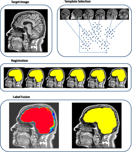
Our method addresses fundamental challenges of multi-atlas approaches. To overcome the difficulties arising from the variability of imaging characteristics between studies, we propose a study-specific template selection strategy, by which we select a set of templates that best represent the anatomical variations within the data set. Against the difficulties of registering brain images with skull, we use a particularly adapted registration algorithm that is more robust to large variations between images, as it adaptively aligns different regions of the two images based not only on their similarity but also on the reliability of the matching between images. Finally, a spatially adaptive weighted voting strategy, which uses the ranking of Jacobian determinant values to measure the local similarity between the template and the target images, is applied for combining coregistered template masks.

Results

The method is validated on three different public data sets and obtained a higher accuracy than recent state-of-the-art brain extraction methods. Also, the proposed method is successfully applied on several recent imaging studies, each containing thousands of magnetic resonance images, thus reducing the manual correction time significantly.

Conclusions

The new method, available as a stand-alone software package for public use, provides a robust and accurate brain extraction tool applicable for both clinical use and large population studies.

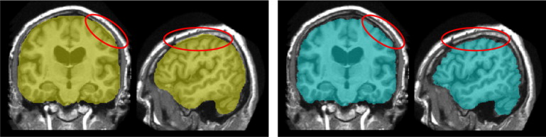
Brain extraction, or skull stripping is a very important preprocessing step preceding almost all automated brain magnetic resonance (MR) imaging (MRI) applications. It consists of the removal of the skull and the extracerebral tissues (e.g., scalp and dura) on brain MR images. An illustrative example of extraction on a T1-weighted image is shown in Figure 1 . Brain extraction is known to be a difficult task, as the boundaries between brain and nonbrain tissues, especially those between the gray matter and the dura matter, might not be clear on MR images. Also, it is more prone to requiring manual intervention as the errors in this step propagate to most subsequent analysis steps, such as registration to a common space, tissue segmentation, cortical thickness and atrophy estimation, etc .

Open full size image

Figure 1

Brain extraction example.

Get Radiology Tree app to read full this article<

Methods

Get Radiology Tree app to read full this article<

Template Selection

Get Radiology Tree app to read full this article<

argmins∑ki=1∑Ij∈Si|xj−μi|2 argmin

∑

∈

−

where xj∈Rd x

∈

ℜ

d is a data vector obtained by concatenating the voxel values of I__j , and the cluster center μi μ

i is the mean of data vectors from images in cluster S__i . We used l 2 -norm as our distance metric. For each cluster, the image closest to the cluster center is selected as the template:

Iti=argminIj∈Si∣∣∣xj−μi∣∣∣2 I

argmin

∈

−

Get Radiology Tree app to read full this article<

Registration

Get Radiology Tree app to read full this article<

Jac(x)=⎛⎝⎜⎜⎜⎜⎜⎜∂h2(x)(∂i)2∂h2(x)∂i∂j∂h2(x)∂i∂k∂h2(x)∂i∂j∂h2(x)(∂j)2∂h2(x)∂j∂k∂h2(x)∂i∂k∂h2(x)∂j∂k∂h2(x)(∂k)2⎞⎠⎟⎟⎟⎟⎟⎟ Jac

(

)

(

∂

(

)

(

∂

)

∂

(

)

∂

(

)

∂

(

)

∂

(

)

(

∂

)

∂

(

)

∂

(

)

∂

(

)

∂

(

)

(

∂

)

and the determinant of this Jacobian matrix is

J(x)=det(Jac(x)). J

(

)

det

(

Jac

(

)

Get Radiology Tree app to read full this article<

Label Fusion

Get Radiology Tree app to read full this article<

Pr(label(u)=1)=∑iRank(Ji(u))⋅label(h−1i(u))∑iRank(Ji(u)) P

(

)

∑

(

)

⋅

(

−

(

)

∑

(

)

where the Rank () operator represents ranking of atlases at each voxel based on the Jacobian determinant value on this voxel. Its value is k if an atlas ranks highest in this voxel, and is ( k + 1 − i ) if an atlas ranks i -th among all atlases. The calculated probability values are thresholded for obtaining a binary brain mask. A threshold value of 0.5 has been used in all validation experiments. This default threshold value could be considered as a “majority voting on weighted votes” assigning the voxel to the label that has more than 50% of the votes after weighting.

Get Radiology Tree app to read full this article<

Postprocessing

Get Radiology Tree app to read full this article<

Data sets

Get Radiology Tree app to read full this article<

Results

Single Registration Comparison

Get Radiology Tree app to read full this article<

D(M,N)=2|M∩N||M|+|N| D

(

)

∩

is a general measure of the segmentation accuracy. It quantifies the amount of overlap between the two binary masks. The Hausdorff distance , the maximal surface-to-surface distance between the two masks, is given as

H(M,N)=max{h(M,N),h(N,M))} H

(

)

max

{

(

)

(

)

}

where

h(M,N)=maxm∈Mminn∈N∥m−n∥ h

(

)

max

∈

min

∈

‖

−

‖

and ∥m−n∥ ‖

−

‖ is the Euclidian distance between the voxels m and n . It is generally used to measure the spatial consistency of the overlap between the two masks. As this metric is very sensitive to noise or local outliers in both masks, we calculated the 95% percentile of the surface-to-surface distance (Hausdorff 95%) as a more robust metric.

Get Radiology Tree app to read full this article<

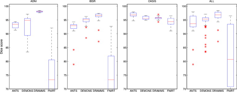
Table 1

Average Dice Scores and 95% of the Surface-to-Surface Distances for within-Group Single-Atlas–Based Brain Extraction Using Four Different Registration Methods

ALL: Images from the three datasets combined.

ANTS DEMONS DRAMMS FNIRT Dice score ADNI 93.1 ± 1.1 92.5 ± 4.6 98.0 ± 0.3 70.6 ± 12.3 IBSR 91.7 ± 3.7 94.6 ± 1.8 95.9 ± 2.5 74.3 ± 8.9 OASIS 96.8 ± 0.9 95.7 ± 0.6 95.7 ± 0.5 94.2 ± 1.6 ALL 93.8 ± 3.1 94.3 ± 3.1 96.5 ± 1.8 79.7 ± 13.6 Hausdorff distance (95%) ADNI 6.05 ± 7.97 11.66 ± 10.69 2.27 ± 2.82 23.79 ± 28.74 IBSR 7.14 ± 7.17 4.78 ± 5.84 4.68 ± 6.71 20.88 ± 36.03 OASIS 3.28 ± 0.98 4.50 ± 0.61 4.3 ± 0.49 5.82 ± 1.52 ALL 5.49 ± 2.89 6.98 ± 6.14 3.75 ± 2.25 16.83 ± 9.89

Get Radiology Tree app to read full this article<

Multi-Atlas Label Fusion

Get Radiology Tree app to read full this article<

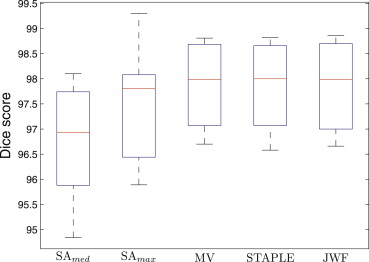
Table 2

Average Dice Scores for Brain Masks Obtained Using Single-Atlas Registration ( SA__med , SA__max ), Multi-Atlas Label Fusion Using Majority Voting (MV), STAPLE, and the Jacobian Determinant-Weighted Label Fusion (JWF)

SA__med__SA__max MV STAPLE JWF ADNI 97.8 ± 0.2 98.1 ± 0.2 98.7 ± 0.1 98.7 ± 0.2 98.7 ± 0.1 OASIS 95.8 ± 0.4 96.5 ± 0.7 97.1 ± 0.2 97.1 ± 0.2 97.0 ± 0.2

Get Radiology Tree app to read full this article<

Comparative Evaluation

Get Radiology Tree app to read full this article<

sensitivity=|TP||N| sensitivity

and

specificity=|TN|∣∣N¯¯¯∣∣ specificity

values between the automatic segmentation M and the ground truth mask N , where the true positive set is defined as TP=M∩N T

∩

N , the true negative set is defined as TN=M¯¯¯¯∩N¯¯¯ T

∩

¯ , and |⋅| |

⋅

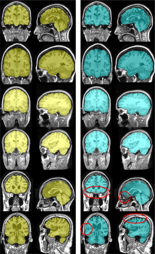
| denotes the number of elements in a set. Table 3 displays the means and standard deviations of the calculated metrics for MASS, BET, and ROBEX.

Table 3

Comparison of MASS to BET and ROBEX on IBSR, OASIS, and LPBA40 Data Sets

Dataset Method Dice Average Distance Hausdorff Hausdorff 95% Sensitivity Specificity IBSR BET 93.8 ± 2.9 2.20 ± 1.20 19.10 ± 9.20 6.20 ± 6.2 99.0 ± 3.5 89.1 ± 2.8 ROBEX 95.6 ± 0.8 1.50 ± 0.30 13.30 ± 2.60 3.80 ± 0.70 99.2 ± 0.5 92.3 ± 1.9 MASS 97.7 ± 0.8 0.71 ± 0.30 15.01 ± 10.72 2.81 ± 1.10 97.5 ± 0.9 99.8 ± 0.2 OASIS BET 93.1 ± 3.7 2.70 ± 1.40 23.70 ± 8.30 8.20 ± 5.50 92.5 ± 5.4 94.2 ± 5.0 ROBEX 95.5 ± 0.8 1.80 ± 0.30 9.80 ± 1.70 4.40 ± 0.60 93.8 ± 2.1 97.4 ± 12.0 MASS 96.1 ± 1.0 1.60 ± 0.36 7.72 ± 1.51 3.81 ± 0.77 94.7 ± 2.6 99.2 ± 0.7 LPBA40 BET 97.3 ± 0.5 1.0 ± 0.20 14.20 ± 4.30 3.0 ± 1.0 97.0 ± 1.3 97.7 ± 0.8 ROBEX 96.6 ± 0.3 1.20 ± 0.10 13.30 ± 2.50 3.10 ± 0.40 95.6 ± 9.0 97.7 ± 7.0 MASS 98.2 ± 0.4 0.66 ± 0.13 9.01 ± 4.07 1.95 ± 0.34 98.2 ± 0.6 99.7 ± 0.2

Get Radiology Tree app to read full this article<

Discussion

Get Radiology Tree app to read full this article<

References

1. Battaglini M., Smith S.M., Brogi S., et. al.: Enhanced brain extraction improves the accuracy of brain atrophy estimation. Neuroimage 2008; 40: pp. 583-589.
2. Zeng X., Staib L.H., Schultz R.T., et. al.: Segmentation and measurement of the cortex from 3D MR images using coupled surfaces propagation. IEEE Transactions on Medical Imaging 1999; 18: pp. 927-937.
3. Shattuck D., Sandor-Leahy S., Schaper K., et. al.: Magnetic resonance image tissue classication using a partial volume model. NeuroImage 2001; 13: pp. 856-857.
4. Huh S., Ketter T.A., Sohn K.H., et. al.: Automated cerebrum segmentation from three-dimensional sagittal brain MR images. Comput Biol Med 2002; 32: pp. 311-328.
5. Smith S.M.: Fast robust automated brain extraction. Hum Brain Mapping 2002; 17: pp. 143-155.
6. Huang A., Abugharbieh R., Tam R., et. al.: MRI brain extraction with combined expectation maximization and geodesic active contours.IEEE International Symposium on Signal Processing and Information Technology.2006.pp. 107-111.
7. Wang Y., Nie J., Yap P.-T., Shi F., Guo L., Shen D.: Robust deformable-surface-based skull-stripping for large-scale studies.Proceedings of the 14th International Conference on Medical Image Computing and Computer-Assisted Intervention: Volume Part III, MICCAI’11.2011.HeidelbergSpringer-Verlag Berlin:pp. 635-642.
8. Carass A., Cuzzocreo J., Wheeler M.B., et. al.: Simple paradigm for extra-cerebral tissue removal: algorithm and analysis. NeuroImage 2011; 56: pp. 1982-1992.
9. Eskildsen S.F., Coupé P., Fonov V., et. al.: Alzheimer’s Disease Neuroimaging Initiative, BEaST: brain extraction based on nonlocal segmentation technique. NeuroImage 2012; 59: pp. 2362-2373.
10. Iglesias J., Liu C.-Y., Thompson P., et. al.: Robust brain extraction across datasets and comparison with publicly available methods. IEEE Trans Med Imaging 2011; 30: pp. 1617-1634.
11. Leung K., Barnes J., Modat M., et. al.: Automated brain extraction using Multi-Atlas Propagation and Segmentation (MAPS).IEEE International Symposium on Biomedical Imaging: From Nano to Macro.2011.pp. 2053-2056.
12. FreeSurfer. http://surfer.nmr.mgh.harvard.edu (sw).
13. AFNI. http://afni.nimh.nih.gov (sw).
14. Mikheev A., Nevsky G., Govindan S., et. al.: Fully automatic segmentation of the brain from T1-weighted MRI using Bridge Burner algorithm. J Magn Reson Imaging 2008; 27: pp. 1235-1241.
15. Sadananthan S., Zheng W., Chee M., et. al.: Skull stripping using graph cuts. NeuroImage 2010; 49: pp. 225-239.
16. Artaechevarria X., Munoz-Barrutia A., Ortiz de Solorzano C.: Combination strategies in multi-atlas image segmentation: application to brain MR data. IEEE Trans Med Imaging 2009; 28: pp. 1266-1277.
17. Isgum I., Staring M., Rutten A., et. al.: Multi-atlas-based segmentation with local decision fusion: application to cardiac and aortic segmentation in CT ccans. IEEE Trans Med Imaging 2009; 28: pp. 1000-1010.
18. Sabuncu M.R., Yeo B., Thomas T., et. al.: A generative model for image segmentation based on label fusion. IEEE Trans Medical Imaging 2010; 29: pp. 1714-1729.
19. Ou Y., Sotiras A., Paragios N., et. al.: DRAMMS: deformable registration via attribute matching and mutual-saliency weighting. Med Image Analysis 2011; 15: pp. 622-639.
20. Jack C., Bernstein M., Fox N., et. al.: The Alzheimer’s Disease Neuroimaging Initiative (ADNI): MRI methods. J Magn Reson Imaging 2008; 27: pp. 685-691.
21. Avants B.B., Epstein C.L., Grossman M., et. al.: Symmetric diffeomorphic image registration with cross-correlation: evaluating automated labeling of elderly and neurodegenerative brain. Med Image Analysis 2008; 12: pp. 26-41.
22. Vercauteren T., Pennec X., Perchant A., et. al.: Diffeomorphic demons: efficient non-parametric image registration. NeuroImage 2009; 1: pp. S61-S72.
23. Andersson J., Smith S., Jenkinson M.: FNIRT—FMRIB non-linear image registration tool.Fourteenth Annual Meeting of the Organization for Human Brain Mapping—HBM.2008.
24. Klein A., Andersson J., Ardekani B., et. al.: Evaluation of 14 nonlinear deformation algorithms applied to human brain MRI registration. NeuroImage 2009; 3: pp. 786-802.
25. Dice L.R.: Measures of the amount of ecologic association between species. Ecology 1945; 26: pp. 297-302.
26. Huttenlocher D.P., Klanderman G.A., Rucklidge W.A.: Comparing images using the hausdorff distance. IEEE Trans Pattern Anal Mach. Intell 1993; 15: pp. 850-863.
27. Warfield S.K., Zou K.H., Wells W.M.: Simultaneous Truth and Performance Level Estimation (STAPLE): an algorithm for the validation of image segmentation. IEEE Trans Med Imaging 2004; 23: pp. 903-921.
28. Sethian J.A.: Level set methods and fast marching methods: evolving interfaces in computational geometry, fluid mechanics, computer vision, and materials science.2nd edition1999.Cambridge University PressUK

Multi-Atlas Skull-Stripping

Rationale and Objectives

Materials and Methods

Results

Conclusions

Methods

Template Selection

Registration

Label Fusion

Postprocessing

Data sets

Results

Single Registration Comparison

Multi-Atlas Label Fusion

Comparative Evaluation

Discussion

References

Further Reading

A Picture Is Worth A Thousand Words

A Retrieval-Based Computer-Aided Diagnosis System for the Characterization of Liver Lesions in CT Scans

Academic Radiology in the New Health Care Delivery Environment