
Rationale and Objectives
Quantitative assessment of knee articular cartilage (AC) morphology using magnetic resonance (MR) imaging requires an accurate segmentation and 3D reconstruction. However, automatic AC segmentation and 3D reconstruction from hydrogen-based MR images alone is challenging because of inhomogeneous intensities, shape irregularity, and low contrast existing in the cartilage region. Thus, the objective of this research was to provide an insight into morphologic assessment of AC using multilevel data processing of multinuclear ( 23 Na and 1 H) MR knee images.
Materials and Methods
A dual-tuned ( 23 Na and 1 H) radio-frequency coil with 1.5-T MR scanner is used to scan four human subjects using two separate MR pulse sequences for the respective sodium and proton imaging of the knee. Postprocessing is performed using customized routines written in MATLAB. MR data were fused to improve contrast of the cartilage region that is further used for automatic segmentation. Marching cubes algorithm is applied on the segmented AC slices for 3D volume rendering and volume is then calculated using the divergence theorem.
Results
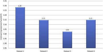
Fusion of multinuclear MR images results in an improved contrast (factor >3) in the cartilage region. Sensitivity (80.21%) and specificity (99.64%) analysis performed by comparing manually segmented AC shows a good performance of the automated AC segmentation. The average cartilage volume (23.19 ± 1.38 cm 3 ; coefficient of variation [COV] −0.059) measured from 3D AC models of four data sets shows a marked improvement over average cartilage volume (23.24 cm 3 ; COV −0.19) reported earlier.
Conclusions
This study confirms the use of multinuclear MR data for cartilage morphology (volume) assessment that can be used in clinical settings.
Osteoarthritis (OA) is one of the most common joint disorders in the knee that affects a large population around the world . Incidences of OA onset have been found in patients with age as early as 25 years . Research in OA assessment involves detection of prediseased to early diseases conditions followed by its monitoring at severe grades. The onset and progression of OA has been associated with the degradation of knee articular cartilage (AC). Changes in physiology and morphology of AC in early stages of diseases progression can be measured by quantitative measurement of selective features that are associated with OA using magnetic resonance (MR) imaging (MRI) .
Morphologic assessment of AC involves measurement of changes in thickness, volume, and curvature . In particular, a decrease in cartilage volume at the rate of ∼5% per year is observed in a longitudinal study of 123 OA patients . In another study, a decrease in volume at ∼2.8% annually is observed in a healthy cartilage . Quantitative measurement of AC morphology (volume and thickness) using MRI is becoming the standard due to its noninvasive nature, nonionizing, and in vivo imaging capabilities. It has been reported that MRI data can be postprocessed for reliable morphologic measurement of the AC in three dimensions (3D). Most of the studies involving morphologic measurement use pre-installed software tools such as Argus, OCTANE Duo, and similar software that are available in most of the MR scanners . These software tools require AC segmentation from MR image slices before 3D rendering and quantitative morphologic assessment. Although the previously described software tools provide regional (by selecting the region of interest manually) assessment of the cartilage morphology, manual segmentation of AC before reconstruct 3D models and manual selection of different cartilage regions are tedious and can result in inter–intra observer issues in the morphologic assessment.
Get Radiology Tree app to read full this article<
Get Radiology Tree app to read full this article<
Get Radiology Tree app to read full this article<
Materials and methods
MRI Data Acquistion
Get Radiology Tree app to read full this article<
Data Preprocessing
Get Radiology Tree app to read full this article<
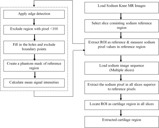
Get Radiology Tree app to read full this article<
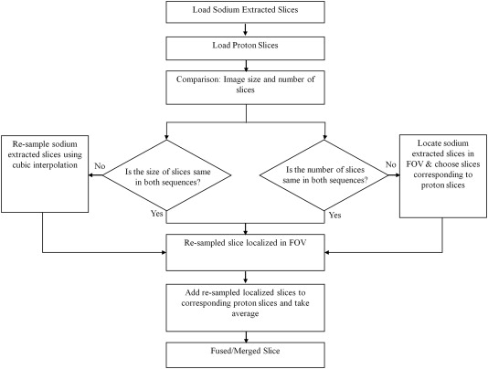
Fusion of Sodium and Proton MR Image
Get Radiology Tree app to read full this article<
Get Radiology Tree app to read full this article<
Get Radiology Tree app to read full this article<
Get Radiology Tree app to read full this article<
C|AC−BG|=1n∣∣∑ni=1IACi−∑nj=1IBGj∣∣ C
|
A
C
−
B
G
|
=
1
n
|
∑
i
=
1
n
I
A
C
i
−
∑
j
=
1
n
I
B
G
j
|
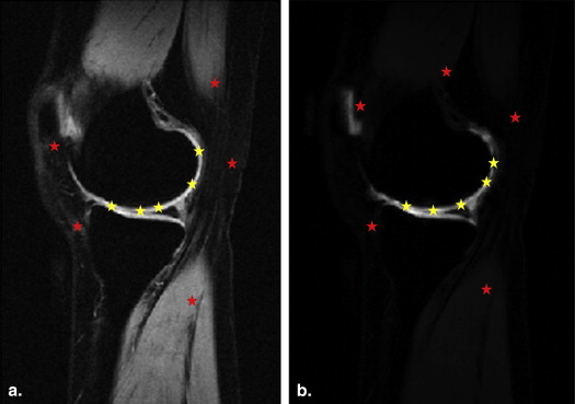
where, I__AC and I__BG represent the intensities in the AC and background regions of fused images, respectively; n is the number of pixels selected in the cartilage and background regions of merged images. Using the same approach, the measured contrast values from fused images are compared to contrast values from original proton slices. In the measurement, five random pixels are selected from the cartilage (yellow dots) and background (red dots) regions of each slice in the data set as shown in Figure 3 , followed by the calculation of mean signal intensities in both regions.
Get Radiology Tree app to read full this article<
Get Radiology Tree app to read full this article<
CIF=CfusedCproton C
I
F
=
C
f
u
s
e
d
C
p
r
o
t
o
n
where, C fused is the contrast difference between the cartilage and background regions of the fused image extracted from sodium and original proton MR images, and C proton is the contrast difference between the cartilage and background regions of original proton images.
Get Radiology Tree app to read full this article<
AC Segmentation
Get Radiology Tree app to read full this article<
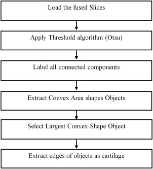
Get Radiology Tree app to read full this article<
Get Radiology Tree app to read full this article<
Sensitivity=TPTP+FN Sensitivity
=
T
P
T
P
+
F
N
Specificity=TNTN+FP Specificity
=
T
N
T
N
+
F
P
where, true positive (TP) is the number of pixels correctly labeled as the cartilage region, true negative (TN) is the number of pixels correctly labeled as the noncartilage region, false positive (FP) is the number of pixels incorrectly labeled as the cartilage region, and false negative (FN) is the number of pixels incorrectly labeled as noncartilage region.
Get Radiology Tree app to read full this article<
3D Reconstruction of AC
Get Radiology Tree app to read full this article<
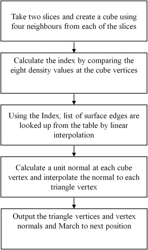
Get Radiology Tree app to read full this article<
Volume Computation of AC
Get Radiology Tree app to read full this article<
Get Radiology Tree app to read full this article<
Get Radiology Tree app to read full this article<
Get Radiology Tree app to read full this article<
V=16∑fi∈F∣∣∣∣∣xi1yi1zi1xi2yi2zi2xi3yi3zi3∣∣∣∣∣where⎧⎩⎨⎪⎪⎪⎪vi1=(xi1,yi1,zi1)vi2=(xi2,yi2,zi2)vi3=(xi3,yi3,zi3) V
=
1
6
∑
f
i
∈
F
|
x
1
i
x
2
i
x
3
i
y
1
i
y
2
i
y
3
i
z
1
i
z
2
i
z
3
i
|
where
{
v
1
i
=
(
x
1
i
,
y
1
i
,
z
1
i
)
v
2
i
=
(
x
2
i
,
y
2
i
,
z
2
i
)
v
3
i
=
(
x
3
i
,
y
3
i
,
z
3
i
)
Get Radiology Tree app to read full this article<
Get Radiology Tree app to read full this article<
∫A∇⋅f→dv=∮∂An→⋅f→dS. ∫
A
∇
⋅
f
→
d
v
=
∮
∂
A
n
→
⋅
f
→
d
S
.
Get Radiology Tree app to read full this article<
Get Radiology Tree app to read full this article<
∇⋅f→=a ∇
⋅
f
→
=
a
where, a a is constant, then the equation can be expressed as
∫Aadv=∮∂An→⋅f→dS. ∫
A
a
d
v
=
∮
∂
A
n
→
·
f
→
d
S
.
Get Radiology Tree app to read full this article<
Get Radiology Tree app to read full this article<
Volume(A)=∫Adv=∮∂An→⋅f→dsa V
o
l
u
m
e
(
A
)
=
∫
A
d
v
=
∮
∂
A
n
→
·
f
→
d
s
a
Get Radiology Tree app to read full this article<
Get Radiology Tree app to read full this article<
∇⋅f→=∂fx∂x+∂fy∂y+∂fz∂z ∇
·
f
→
=
∂
f
x
∂
x
+
∂
f
y
∂
y
+
∂
f
z
∂
z
where, f→=(fx,fy,fz)T f
→
=
(
f
x
,
f
y
,
f
z
)
T
Get Radiology Tree app to read full this article<
Get Radiology Tree app to read full this article<
∫A∂x∂x+∂y∂y+∂z∂zdv=∮∂An→⋅f→dS ∫
A
∂
x
∂
x
+
∂
y
∂
y
+
∂
z
∂
z
d
v
=
∮
∂
A
n
→
·
f
→
d
S
∫A3dv=∮∂An→⋅f→dS ∫
A
3
d
v
=
∮
∂
A
n
→
·
f
→
d
S
Get Radiology Tree app to read full this article<
Get Radiology Tree app to read full this article<
Volume(A)=∫Adv=∮∂An→⋅f→dS3 V
o
l
u
m
e
(
A
)
=
∫
A
d
v
=
∮
∂
A
n
→
·
f
→
d
S
3
Get Radiology Tree app to read full this article<
Results
Data Acquisition and Preprocessing
Get Radiology Tree app to read full this article<
Get Radiology Tree app to read full this article<
Get Radiology Tree app to read full this article<
Get Radiology Tree app to read full this article<
Fusion of Proton and Sodium Extracted Slices
Get Radiology Tree app to read full this article<
Get Radiology Tree app to read full this article<
Get Radiology Tree app to read full this article<
Table 1
Mean Signal Intensity Values Obtained From Background and the Cartilage Region of Original Proton and Fused Slices
Data Set Proton Data Set Fused Data Set Average MSI BG Average MSI AC C Proton Average MSI BG Average MSI AC C Fused Data set 1 117.74 148.05 30.32 66.62 166.19 99.56 Data set 2 146.84 182.78 35.94 61.29 174.44 113.15 Data set 3 130.14 161.07 30.93 67.65 161.24 93.58 Data set 4 145.79 178.76 32.97 65.30 169.18 103.88
AC, articular cartilage; C Fused , contrast difference between articular cartilage and background of fused images; C Proton , contrast difference between articular cartilage and background of proton images; MSI AC , mean signal intensities in articular cartilage region; MSI BG , mean signal intensities in background region.
Get Radiology Tree app to read full this article<
Get Radiology Tree app to read full this article<
Get Radiology Tree app to read full this article<
Automatic Segmentation of AC
Get Radiology Tree app to read full this article<
Get Radiology Tree app to read full this article<
Get Radiology Tree app to read full this article<
Table 2
Sensitivity and Specificity Analysis Through a Comparison Between Automatically Segmented Slices and Manually Segmented Slices by Two Observers
Data Sets Observer 1 Observer 2 Sensitivity Specificity Sensitivity Specificity Data set 1 80.27 99.65 79.53 99.68 Data set 2 79.13 99.46 80.77 99.57 Data set 3 89.34 99.72 90.17 99.69 Data set 4 72.08 99.74 74.79 99.78 SD 7.082 0.12 6.44 0.08 Average 80.20 99.64 81.31 99.68 COV 0.088 0.0012 0.079 0.0008
COV, coefficient of variation; SD, standard deviation.
Get Radiology Tree app to read full this article<
3D Reconstruction and Volume Computation
Get Radiology Tree app to read full this article<
Get Radiology Tree app to read full this article<
Get Radiology Tree app to read full this article<
Get Radiology Tree app to read full this article<
Table 3
Average, Standard Deviation, and Coefficient of Variation Values for Total Cartilage Volume Calculation in Different Data Sets
Data Sets TCV 3Dautomatic (mm 3 ) TCV 3Dmanualfirst (mm 3 ) TCV 3Dmanualsecond (mm 3 ) Error (%) Data set 1 22,430 16,585 18,329 −28.48 Data set 2 22,425 18,756 18,736 −19.62 Data set 3 25,268 22,539 24,000 −8.58 Data set 4 22,667 23,504 23,297 3.13 SD 1384 3238 2972 Average 23,197 20,346 21,091 COV 0.0596 0.1591 0.1409
COV, coefficient of variation; SD, standard deviation; TCV 3Dautomatic , total cartilage volume in 3D model reconstructed from automatically segmented cartilage; TCV 3Dmanualfirst , total cartilage volume in 3D model reconstructed from segmented cartilage by first observer; TCV 3Dmanualsecond , total cartilage volume in 3D model reconstructed from segmented cartilage by second observer.
Get Radiology Tree app to read full this article<
Get Radiology Tree app to read full this article<
Get Radiology Tree app to read full this article<
Discussion
Get Radiology Tree app to read full this article<
Acknowledgment
Get Radiology Tree app to read full this article<
Get Radiology Tree app to read full this article<
References
1. Akinpelu A.O., Alonge T.O., Adekanla B.A., et. al.: Prevalence and pattern of symptomatic knee osteoarthritis in Nigeria: a community-based study. Internet Journal of Allied Health Sciences and Practice 2009; 7:
2. W. P. Lubar D, Callahan LF, Chang RW, et al. A National Public Health Agenda for Osteoarthritis 2010. Centers for Disease Control and Prevention, USA. Available: URL: http://www.arthritis.org/media/Ad%20Council%20101/OA_Agenda_2010.pdf
3. Hani A.F.M., Malik A.S., Kumar D., et al. Features and modalities for assessing early knee osteoarthritis. International Conference onElectrical Engineering and Informatics (ICEEI), 2011; vol., no., pp.1–6, 17-19 July 2011.
4. Hani A.F.M., Kumar D., Malik A.S., et. al.: Physiological assessment of in vivo human knee articular cartilage using sodium MR imaging at 1.5 T. Magnetic Resonance Imaging September 2013; 31: pp. 1059-1067.
5. Eckstein F., Cicuttini F., Raynauld J.P., et. al.: Magnetic resonance imaging (MRI) of articular cartilage in knee osteoarthritis (OA): morphological assessment. Osteoarthritis and Cartilage 2006; 14: pp. 46-75.
6. Wluka A.E., Stuckey S., Snaddon J., et. al.: The determinants of change in tibial cartilage volume in osteoarthritic knees. Arthritis and Rheumatism August 2002; 46: pp. 2065-2072.
7. Hanna F., Ebeling P.R., Wang Y., et. al.: Factors influencing longitudinal change in knee cartilage volume measured from magnetic resonance imaging in healthy men. Ann Rheum Dis 2005; 64: pp. 1038-1042.
8. Maataoui A., Graichen H., Abolmaali N.D., et. al.: Quantitative cartilage volume measurement using MRI: comparison of different evaluation techniques. EurRadiol 2005; 15: pp. 1550-1554.
9. J CarballidoGamio, JS. Bauer, K-Y Lee, et al. Combined image processing techniques for characterization of MRI cartilage of the knee.Proc. 27th Annual Conf. IEEE Engineering in Medicine and Biology, Shanghai, China, 2005, pp.3043–pp.3046
10. Swamy M.M.S., Holi M.S.: Knee joint articular cartilage segmentation, visualization and quantification using image processing techniques: a review. International Journal of Computer Applications March 2012; 42: pp. 36-43.
11. Swamy M.M.S., Holi M.S.: Knee joint articular cartilage segmentation using radial search. Method, visualization and quantification. International Journal of Biometrics and Bioinformatics (IJBB) 2013; 7:
12. Hani, A.F.M.; Kumar, D.; Malik, A.S, et al. Fusion of multinuclear magnetic resonance images of knee for the assessment of articular cartilage. Engineering in Medicine and Biology Society (EMBC), 2013 35th Annual International Conference of the IEEE, vol., no., pp.6466, 6469, 3–7 July 2013
13. Koo S., Hargreaves B.A., Andriacchi T.P., et. al.: Automatic segmentation of articular cartilage from MRI: a multi-contrast and multi-dimensional approach. Proc. Intl. Soc. Mag. Reson. Med 2008; 16: pp. 2546.
14. Hani A.M., Kumar D., Malik A., et. al.: Non-invasive sodium MR imaging and quantification of in-vivo articular cartilage at 1.5 tesla. Osteoarthritis and Cartilage April 2012; 20: pp. S18-S19.
15. Hani, A Fadzil M; Kumar, D; Malik, AS. Performance evaluation of dual tuned knee coil ( 23 Na/ 1 H) for articular cartilage imaging on 1.5Tesla MRI.4th International Conference onIntelligent and Advanced Systems (ICIAS) 2012 vol. 1, pp.357,361, 12–14 June 2012
16. Mohd Hani A., Kumar D., Malik A., et. al.: Accessibility to combined assessment of morphology and physiology in articular cartilage using 23NA/1H coil at 1.5 Tesla MRI. Osteoarthritis and Cartilage 2013; 21: pp. S192-S193.
17. Mohd Hani A., Kumar D., Malik A., et. al.: Automatic segmentation of articular cartilage from combined assessment of sodium and proton MR knee images. Osteoarthritis and Cartilage 2013; 21: pp. S198-S199.
18. Pakin S.K., Tamez-Pena J.G., Totterman S., et. al.: Segmentation, surface extraction and thickness computation of articular cartilage. SPIE 2002; 4684: pp. 155-166.
19. Warfield S.K., Kaus M., Jolesz F.A., et. al.: Adaptive, template moderated, spatially varying statistical classification. Medical Image Analysis 2000; pp. 43-55.
20. Fazel S.A.A., Gal Y., Yang Z., et. al.: Qualitative and quantitative analysis of six image fusion methodologies and their application to medical imaging. Proc. International Conference on Digital Image Computing: Techniques and Applications 2011;
21. Lorensen W.E., Cline H.E.: Marching cubes: a high resolution 3D surface construction algorithm. ACM Computer Graphics 1987; 21: pp. 163-169.
22. Baysal O., Baysal T., Alkan A., et. al.: Comparison of MRI graded cartilage and MRI based volume measurement in knee osteoarthritis. SWISS MED WKLY 2004; 134: pp. 283-288.
23. Cicuttini F., Forbes A., Morris K., et. al.: Gender differences in knee cartilage volume as measured by magnetic resonance imaging. Osteoarthritis Cartilage 1999 May; 7: pp. 265-271.
24. Trinh N.H., Lester J., Fleming B.C., et. al.: Accurate measurement of cartilage morphology using a 3D laser scanner. Computer Vision Approaches to Medical Image Analysis, Lecture Notes in Computer Science 2006; 4241: pp. 37-48.
25. Eckstein F., Winzheimer M., Westhoff J., et. al.: Quantitative relationships of normal cartilage volumes of the human knee joint–assessment by magnetic resonance imaging. AnatEmbryol (Berl) 1998 May; 197: pp. 383-390.
26. Wang S.: “3D volume calculation for the Marching cubes algorithm in cartesian coordinates.” Numerical analysis (math.NA).June, 2013.Cornell University Library Retrieved http://xxx.tau.ac.il/pdf/1308.0387.pdf