Rationale and Objectives

We present a model for the optimal placement of mono- and bipolar probes in radiofrequency (RF) ablation. The model is based on a system of partial differential equations that describe the electric potential of the probe and the steady state of the induced heat distribution.

Materials and Methods

To optimize the probe placement we minimize a temperature-based objective function under the constraining system of partial differential equations. Further, the extension of the resulting optimality system for the use of multiple coupled RF probes is discussed. We choose a multiscale gradient descent approach to solve the optimality system.

Results

This article describes the discretization and implementation of the approach with finite elements on three-dimensional hexahedral grids.

Conclusion

Applications of the optimization to artificial test scenarios as well as a comparison to a real RF ablation show the usefulness of the approach.

During the last decade, local and minimally invasive techniques have become a promising treatment of tumor diseases. Especially in situations in which a surgical resection or chemotherapy is not possible because of the extent of the tumor or the general state of the patient, thermotherapies such as radiofrequency (RF) ablation offer an alternative and less invasive form of treatment.

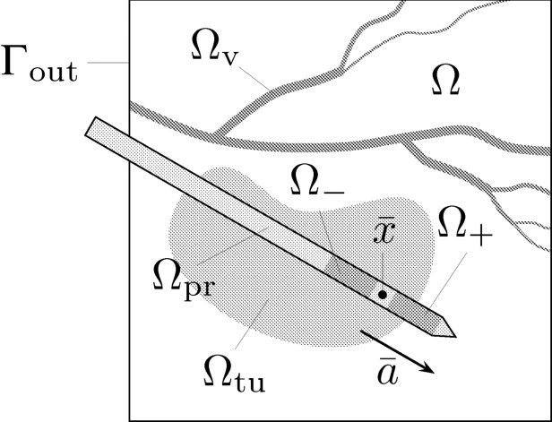
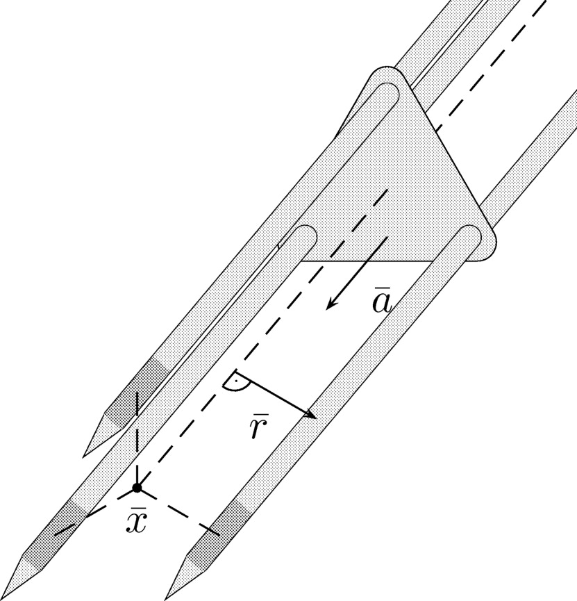
In this work, we consider the RF ablation of hepatic tumors with mono- or bipolar systems (see Fig 1 ): A probe, which is connected to an electric generator, is placed inside the malignant tissue, so that an electric current flows through the body and heats the tissue near the probe up to temperatures of more than 60°C.

Open full size image

Figure 1

Schematic sketch of a bipolar RF ablation.

Get Radiology Tree app to read full this article<

A model for the simulation of RF ablation

Get Radiology Tree app to read full this article<

−div(σ∇)=0inΩ\Ω¯¯¯± −

div

(

∇

)

with appropriate boundary conditions (see below), models the electric potential ϕ : Ω → R of the RF probe. Here, σ ∈ ℝ is the electric conductivity of the tissue. For the electrostatic equation, we consider the boundary conditions

=±1onΩ¯¯¯+andΩ¯¯¯−,

and

−

n⋅∇=n⋅(x¯−x)|x¯−x|2onΓout, n

⋅

∇

⋅

(

−

)

−

out

where n denotes the outer normal on Γ out . Equation 2a fixes the potential on the electrodes, and the Robin boundary condition in Eq 2b is based on the assumption that on the boundary (far from the probe) the potential behaves approximately as induced by a point load at the barycenter x¯ x

¯ of the probe.

Get Radiology Tree app to read full this article<

R=U2PtotalwithPtotal=∫Ωσ|∇|2dx, R

total

with

total

∫

∇

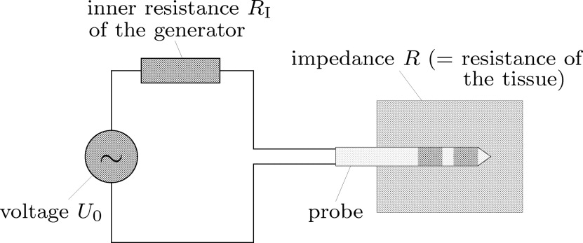
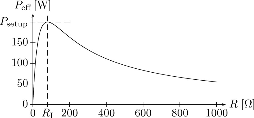
where U is the difference of the potential ϕ on the two electrodes ( U = 2V for bipolar probes and U = 1V for monopolar probes) (see Eq 2a ). According to the equivalent circuit diagram shown in Fig 2 , the effective power of the generator is now given by

Peff=4PsetupRRI(R+RI)2, P

eff

setup

(

)

where R I is the inner resistance of the generator and P setup is the value set up at the generator’s control unit. Finally, the heat source is given by

Qrf=PeffPtotalσ|∇|2. Q

eff

total

∇

The spatial distribution of heat T : Ω → ℝ is modeled by the steady state of the so-called bioheat-transfer equation

−div(λ∇T)=Qrf+QperfinΩ. −

div

(

∇

)

perf

Here, λ ∈ ℝ is the thermal conductivity of the tissue. The right hand side of Eq 3 consists of the source (heating) Q rf from the electric current and the sink (cooling) Q perf from the vascular system. We assume that there is no heating on the outer boundary of Ω and thus consider the Dirichlet boundary condition

T=TbodyonΓout. T

body

out

Finally, the term modeling the cooling effects of the blood perfusion Q perf is a variant of the approach of Pennes ( ):

Qperf=−v(T−Tbody), Q

perf

−

(

−

body

)

where

v=v(x)={vvesselρm,Bcm,B,vcapρm,Bcm,B,x∈Ωv,else. v

(

)

{

vessel

m,B

∈

cap

m,B

else

Thus the coefficient v depends on the relative blood circulation rate vvessel[s−1] v

vessel

[

−

] of vessels and vcap[s−1] v

cap

[

−

] of capillaries respectively, as well as on the blood density ρ m,B [k g /m] and the heat capacity cm,B[J/kgK] c

m,B

[

] of blood. Here we assume that the whole tissue is pervaded by capillary vessels and thus is exposed to their cooling influence.

Get Radiology Tree app to read full this article<

−σΔ=0inΩ/Ω¯¯¯±, −

σΔ

−λΔT+vT=Qrf+vTbodyinΩ −

λΔT

body

with boundary conditions Eq 2a, 2b, and 4 . Here H 1 = H 1,2 denotes the Sobolev space of functions having weak derivatives ( ). Note that the two equations are coupled through the term Q rf on the right hand side of the steady state heat equation in Eq 5b .

Get Radiology Tree app to read full this article<

Objective functions

Get Radiology Tree app to read full this article<

f(T)=ω12∥T−Tbody∥2L2(Ω\Ωtu)+ω22∥T−Tcrit∥2L2(Ωtu) f

(

)

∥

−

body

∥

(

)

∥

−

crit

∥

(

)

with ω 1 and ω 2 being suitable weights, so that the above requirements are met. Here, L 2 (Ω) is the space of square integrable functions on Ω and ∥∥v∥2L2=(v,v) ∥

∥

(

) is the norm on L 2 where ( v,w ) = ∫ Ω vwdx denotes the scalar poduct.

Get Radiology Tree app to read full this article<

f(T)=∫Ωtue−T(x)dx. f

(

)

∫

−

(

)

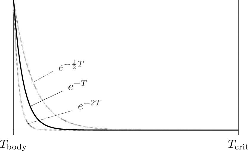
By using the exponential function, we aim at an equal heat distribution inside the tumor. The lowest temperature inside the tumor is penalized most (see black curve in Fig 5 ), so that configurations with only a small sufficiently hot volume inside the tumor lead to a higher value of the objective function than a uniform tumor heating.

Get Radiology Tree app to read full this article<

f(T)=∫Ωtue−αT(x)dx. f

(

)

∫

−

(

)

This allows for a modification of the grade of penalization of a non-uniform temperature distribution inside the tumor (lower penalization for α < 1; stronger penalization for α > 1; see gray curves in Fig 4 ).

Get Radiology Tree app to read full this article<

f(T)=eTmin∫Ωtue−T(x)dx=∫ΩtueTmin−T(x)dx, f

(

)

min

⁡

∫

−

(

)

∫

min

⁡

−

(

)

where T min is the minimal temperature of the current iteration step. This modification guarantees that the argument of the exponential function does not become too large. The analog modification for the objective function ( ) is straightforward.

Get Radiology Tree app to read full this article<

Optimizing the probe placement

Get Radiology Tree app to read full this article<

Qrf=Q(u),Q:U→L2(Ω),T=T(Qrf),T:L2(Ω)→H1(Ω) Q

(

)

→

(

)

(

)

(

)

→

(

)

To optimize the probe location, we are looking for u ∈ U such that F:U→R,u↦F(u):=f F

→

ℝ

↦

(

)

f · T T · Q Q ( u ) becomes minimal.

Get Radiology Tree app to read full this article<

U˜=Ω×(R3{0})⊃U, U

(

ℝ

{

}

)

⊃

and introduce the projection

P:U˜→U,(x¯,a¯)↦(x¯,a¯/|a¯|). P

→

(

)

↦

(

)

Now we set

Q(x¯,a¯)=(Q⋅P)(x¯,a¯)=Q(x¯,a¯/|a¯|), Q

(

)

(

⋅

)

(

)

(

)

(ie, Q Q does not depend on the length of a¯ a

¯ ).

Get Radiology Tree app to read full this article<

Initial value

Get Radiology Tree app to read full this article<

Descent direction

Get Radiology Tree app to read full this article<

Step size

Get Radiology Tree app to read full this article<

Stopping criterion

Get Radiology Tree app to read full this article<

Descent Direction

Get Radiology Tree app to read full this article<

∂ujF(u)=f′(T⋅Q(u))[T′(Q(u))[∂ujQ(u)]]=T′(Q(u))*[f′(T⋅Q(u))][∂ujQ(u)] ∂

(

)

′

(

⋅

(

)

[

′

(

)

[

∂

(

)

]

′

(

)

[

′

(

⋅

(

)

]

[

∂

(

)

]

where ′ denotes the Frechet derivative, * denotes the adjoint operator, and brackets [ · ] denote the application of linear operators. For the calculation of ∂ujQ(u) ∂

(

) , we use a numerical approximation by central differences, whereas we determine f′ analytically as

f′(T)[w]=−(αe−αT,w)L2(Ωtu). f

′

(

)

[

]

−

(

−

)

(

)

Get Radiology Tree app to read full this article<

T′(Qrf)*[f′(T)][w]=(p,w)L2(Ω), T

′

(

)

[

′

(

)

]

[

]

(

)

(

)

where p ∈ H 1 (Ω) is the solution to the adjoint problem of Eq 5b with boundary condition (Eq 4 ):

−λΔp+vp=−αe−αTp=0inΩ,onΓout. −

−

out

The advantage of the above application of the chain-rule Eq 8 over a numerical approximation of ∂ujF(u) ∂

(

) is the reduction of the numerical effort. Our approach needs evaluations of the potential equation only (everything else is done analytically), whereas a full numerical differentiation would involve the coupled system (Eq 5a, 5b ) and thus be at least about twice as expensive.

Get Radiology Tree app to read full this article<

Step Size

Get Radiology Tree app to read full this article<

s0∣∣v0∣∣=12diam(Ω),i.e.s0=diam(Ω)2|v0|. s

diam

(

)

i.e.

diam

(

)

In the following iteration steps n > 0 we start with a step size that fulfills

|vn|sn=2∣∣vn−1∣∣sn−1,i.e.sn=2∣∣vn−1∣∣|vn|sn−1. |

−

i.e.

−

After having chosen an initial value for the step size s n , we bisect s n until the new iterate un+1=P(un+snvn) u

(

) fulfills u__n +1 ∈ U and F( u__n +1 ) < F ( u__n ). If these conditions are not matched after a certain number of bisections, the step size s n is set to zero and the algorithm stops.

Get Radiology Tree app to read full this article<

Stopping Criterion

Get Radiology Tree app to read full this article<

∣∣x¯n+1−x¯n∣∣<1and∣∣a¯n+1−a¯n∣∣<2. |

−

and

−

Get Radiology Tree app to read full this article<

Optimization of Multiple Coupled Probes

Get Radiology Tree app to read full this article<

U={(x¯,a¯,r¯)∈Ω×S2×S2:r¯⊥a¯}. U

{

(

)

∈

⊥

}

Again, for easier handling of the gradient with respect to the optimization variable, we replace U with the open set

U˜={(x¯,a¯,r¯)∈Ω×R3×R3:r¯∦a¯} U

{

(

)

∈

ℝ

∦

}

and use the projection

P:U˜→U,(x¯,a¯,r¯)↦(x¯,a¯|a¯|,|a¯|2r¯−(r¯,a¯)a¯||a¯|2r¯−(r¯,a¯)a¯∣∣). P

→

(

)

↦

(

−

(

)

−

(

)

Get Radiology Tree app to read full this article<

Discretization with finite elements

Get Radiology Tree app to read full this article<

Reduction to a Linear System of Equations

Get Radiology Tree app to read full this article<

λ(∇T,∇v)L2(Ω)+v(T,v)L2(Ω)=(Qrf+vTbody,v)L2(Ω)∀v∈H10(Ω). λ

(

∇

)

(

)

(

)

(

)

(

body

)

(

)

⁢

∀

∈

(

)

Get Radiology Tree app to read full this article<

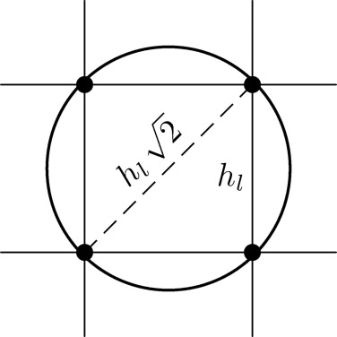
Vhl=span{ψli|i=1,…,nl}, V

span

{

…

}

where ψli ψ

l is given by the requirements that ψli ψ

l is trilinear on each grid cell of G l and ψli(xj)=δij ψ

(

)

j for all nodes xi∈Nl x

⁢

∈

l . Here δ ij is the Kronecker symbol. Then every function w∈Vhl w

⁢

∈

h is determined by its nodal values w i at the vertices x i ∈ N l :

w(x)=∑nli=1wiψli(x). w

(

)

∑

(

)

Because the weak form (Eq 11 ) is linear in the test function v , it suffices to test this equation with all the basis functions of Vhl V

h (ie v = ψil ψ

i for j = 1, …, n l ). This leads to a system of equations in the nodal values t i of the temperature T . Denoting the vector of nodal values with t = ( t i ) i and the right hand side with r = ( r i ) i , we have to solve

(λL+M)t=rwithri=(Qrf+vTbody,ψli)L2(Ω), (

λL

)

⁢

with

⁢

(

body

)

(

)

where L = ( L ij ) ij is the so called stiffness matrix and M = ( M ij ) ij the so called mass matrix defined by

Lij=(∇ψli,∇ψlj)L2(Ω)andMij=(vψli,ψlj)L2(Ω). L

(

∇

)

(

)

and

(

)

(

)

Get Radiology Tree app to read full this article<

Numerical Integration

Get Radiology Tree app to read full this article<

∫Ωtue−αT(x)dx=∑E∈Gl∫EχLtu(x)e−αT(x)dx≈∑E∈Gl|E|8∑xi∈E∩Nl(χLtue−αT)(xi). ∫

−

(

)

∑

∈

∫

(

)

−

(

)

≈

∑

∈

∑

∈

∩

(

−

)

(

)

For the integration of the mass matrix M and the right hand side r , we use lumped masses ( ), which corresponds to a quadrature in which the coefficient v and the heat source Q rf are evaluated at the midpoints of elements only.

Get Radiology Tree app to read full this article<

A Multiscale Optimization Approach

Get Radiology Tree app to read full this article<

Rll+1:Vhl+1→Vhl R

⁢

→

for l = 0, …, L − 1, which transports finite element functions to the next coarser level. A straightforward approach would use the trivial restriction that directly multiplies the nodal values of a fine-grid function with the coarse-grid basis function. However, this leads to unsatisfactory results, because on coarse grids it does not preserve details of the tumor, which have important influence on the choice of the optimal probe positioning. Therefore we propose to use the classical restriction of multigrid approaches for the solution of PDEs ( ). We set Rll+1=(Pll+1)T R

(

)

T where Pll+1 P

l is the trilinear interpolation from grid G l to grid G l +1 involving the weights {1/8,1/4,1/2,1}. So we set

χltu=Rll+1χl+1tu,χlv=Rll+1χl+1v. χ

Get Radiology Tree app to read full this article<

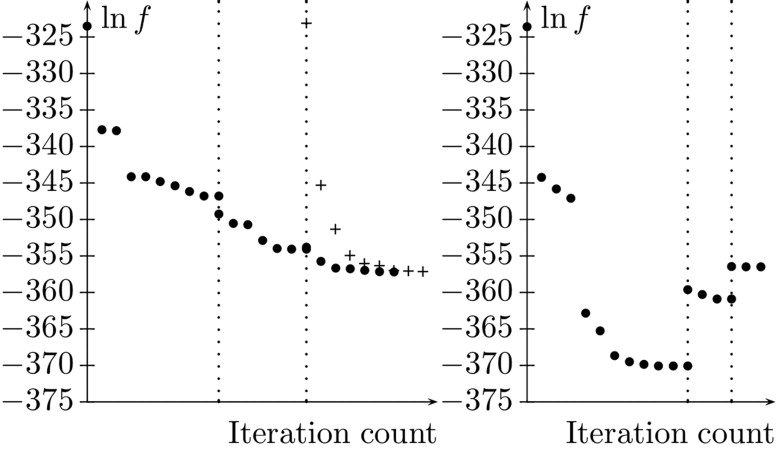
χltu(xj)={10if(Rll+1χl+1)(xj)≥1/2else, χ

(

)

{

(

)

(

)

≥

else,

and analog for χlv χ

l . The progression of the corresponding objective function value is shown in the right graph of Fig 7 . Because here the mass of the tumor and the vessels is not conserved on the coarse levels, the values of the objective function increase at the transition stages.

Get Radiology Tree app to read full this article<

The Optimization Algorithm

Get Radiology Tree app to read full this article<

Table 1

Algorithm 1—Multi-scale optimization of the probe location

1:l ← l 0 ▷Start with level l 0 2: Initialize u¯. u

. 3:while l ≤ L do 4:u 0 ← u¯ u

¯ ▷ Initialization 5:n ← 0 6:repeat ▷ Compute descent direction 7:v n ← −∇ u__F ( u n ) 8:if n = 0 then ▷ Initialize step size 9:s 0 = (2| v 0 |) −1 diam(Ω) 10:else 11:s n = 2| v__n −1 |(| v n |) −1 s__n −1 12:end if 13:m ← 0 ▷ Reset counter ▷ Determine step size 14:u__n +1 ← P ( u n + s n v n ) 15:while F ( u__n +1 ) > F ( u n ) or u__n +1 ∉ U do 16:m ← m + 1 ▷ Increase counter 17:if m = m max then 18: STOP. 19:end if 20:s n ← s n /2 ▷ Bisect step size 21:u__n +1 ← P ( u n + s n v n ) 22:end while 23:until u n +1 − u n | ≤ θ 24:u¯ u

¯ ← u__n +1 25:l ← l + 1 ▷ Proceed to next level 26:end while

Get Radiology Tree app to read full this article<

Numerical results

Get Radiology Tree app to read full this article<

Conclusions and future work

Get Radiology Tree app to read full this article<

Acknowledgments

Get Radiology Tree app to read full this article<

References

1. Stein T.: Untersuchungen zur Dosimetrie der hochfrequenzstrominduzierten interstitiellen Thermotherapie in bipolarer Technik, vol 22.2000.Müller and Berlien Fortschritte in der Lasermedizin
2. Tungjitkusolum S., Staelin S.T., Haemmerich D., et. al.: Three-dimensional finite-element analyses for radio-frequency hepatic tumor ablation. IEEE Trans Biomed Eng 2002; 49: pp. 3-9.
3. Welp C., Siebers S., Ermert H., et. al.: Investigation of the influence of blood flow rate on large vessel cooling in hepatic radiofrequency ablation. Biomed Tech 2006; 51: pp. 337-346.
4. Deuflhard P., Weiser M., Seebaß M.: A new nonlinear elliptic multilevel FEM applied to regional hyperthermia. Comp Vis Sci 2000; 3: pp. 115-120.
5. Roggan A. Dosimetrie thermischer Laseranwendungen in der Medizin 1997; 16 (Fortschritte in der Lasermedizin, Müller and Berlien, 1997.
6. Jain M.K., Wolf P.D.: A three-dimensional finite element model of radiofrequency ablation with blood flow and its experimental validation. Ann Biomed Eng 2000; 28: pp. 1075-1084.
7. Preusser T., Weihusen A., Peitgen H.O.: On the modelling of perfusion in the simulation of RF-ablation. SimVis 2005; pp. 259-269.
8. Tröltzsch F.: Optimale Steuerung partieller Differentialgleichungen.2005.ViewegWiesbaden
9. Geiger C., Kanzow C.: Theorie und Numerik restringierter rungsaufgaben.2002.SpringerBerlin
10. Khalil-Bustany I.S., Diederich C.J., Polak E., et. al.: Minmax optimization-based inverse treatment planning for interstitial thermal therapy. Int J Hypertherm 1998; 14: pp. 347-366.
11. Gaenzler T., Volkwein S., Weiser M.: SQP methods for parametric identification problems arising in hyperthermia. Optimization Methods Software 2006; 6: pp. 869-887.
12. Villard C., Soler L., Gangi A.: Radiofrequency ablation of hepatic tumors: simulation, planning, and contribution of virtual reality and haptics. Comp Meth Biomech Biomed Eng 2005; 8: pp. 215-227.
13. Bourquain H., Schenk A., et. al.: Hepavision2: a software assistant for preoperative planning in living-related liver transplantation and oncologic liver surgery. CARS 2002; pp. 341-346.
14. Pennes H.H.: Analysis of tissue and arterial blood temperatures in a resting forearm. J Appl Physiol 1948; 1: pp. 93-122.
15. Altrogge I., Kröger T., Preusser T., et. al.: Towards optimization of probe placement for radio-frequency ablation. LNCS 2006; 4190: pp. 486-493.
16. Braess D.: Finite Elemente, ed 3.2003.SpringerBerlin:
17. Preusser T., Rumpf M.: An adaptive finite element method for large scale image processing.1999.pp. 223-234.
18. Thomee V.: Galerkin-finite element methods for parabolic problems.1984.SpringerNew York
19. Hackbusch W.: Multi-grid methods and applications, Vol. 4 of Springer Series in Computational Mathematics.1985.SpringerBerlin

Multiscale Optimization of the Probe Placement for Radiofrequency Ablation

Rationale and Objectives

Materials and Methods

Results

Conclusion

A model for the simulation of RF ablation

=±1onΩ¯¯¯+andΩ¯¯¯−,

Objective functions

Optimizing the probe placement

Initial value

Descent direction

Step size

Stopping criterion

Descent Direction

Step Size

Stopping Criterion

Optimization of Multiple Coupled Probes

Discretization with finite elements

Reduction to a Linear System of Equations

Numerical Integration

A Multiscale Optimization Approach

The Optimization Algorithm

Numerical results

Conclusions and future work

Acknowledgments

References

Further Reading

Abstracts of Funded National Institutes of Health Grants

Academic Technology Transfer and Radiology

Advances in Radiologic Image Analysis From MICCAI 2006