Multivariate Normally Distributed Biomarkers Subject to Limits of Detection and Receiver Operating Characteristic Curve Inference

Rationale and Objectives

Biomarkers are of ever-increasing importance to clinical practice and epidemiologic research. Multiple biomarkers are often measured per patient. Measurement of true biomarker levels is limited by laboratory precision, specifically measuring relatively low, or high, biomarker levels resulting in undetectable levels below, or above, a limit of detection (LOD). Ignoring these missing observations or replacing them with a constant are methods commonly used although they have been shown to lead to biased estimates of several parameters of interest, including the area under the receiver operating characteristic (ROC) curve and regression coefficients.

Materials and Methods

We developed asymptotically consistent, efficient estimators, via maximum likelihood techniques, for the mean vector and covariance matrix of multivariate normally distributed biomarkers affected by LOD. We also developed an approximation for the Fisher information and covariance matrix for our maximum likelihood estimations (MLEs). We apply these results to an ROC curve setting, generating an MLE for the area under the curve for the best linear combination of multiple biomarkers and accompanying confidence interval.

Results

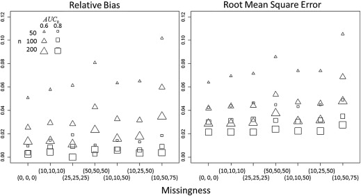
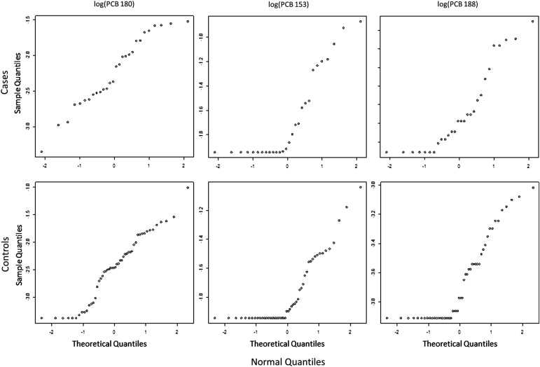
Point and confidence interval estimates are scrutinized by simulation study, with bias and root mean square error and coverage probability, respectively, displaying behavior consistent with MLEs. An example using three polychlorinated biphenyls to classify women with and without endometriosis illustrates how the underlying distribution of multiple biomarkers with LOD can be assessed and display increased discriminatory ability over naïve methods.

Conclusions

Properly addressing LODs can lead to optimal biomarker combinations with increased discriminatory ability that may have been ignored because of measurement obstacles.

The use of biomarkers, including medical images, is becoming increasingly common in the diagnosis and prognosis of individuals with a given disease in clinical settings and epidemiologic research. Combining various sources of biologic information quantitatively, through diagnostic indices for example, allows a concrete way to collapse blood, imaging, and other biomarker information. The receiver operating characteristic (ROC) curve is a tool frequently used to assess the usefulness of biomarkers as diagnostic tools . Some biomarkers, often emerging ones, are difficult to measure and/or are measured with less than optimally refined laboratory methods, making it difficult to assess any potential clinical usefulness. Specifically, limits of quantifiable biomarker levels are introduced by the sensitivity of the measurement instrument or process, which often leads to censored measurements at either the lower or upper end of the biomarker spectrum. The points at which this censoring occurs are called the limit of detection (LOD) and point of saturation, respectively . However, scientists remain interested in the biomarkers’ potential relations, causations, and discriminatory ability for adverse outcomes and disease despite this measurement-induced error of censoring. For instance, polychlorinated biphenyl (PCB) levels are a group of compounds that have been linked with several adverse outcomes but their correlated nature and measurements being affected by LODs have hindered their study.

Consider p biomarkers that are of interest in a particular population, where each individuals has true values for each, denoted by W−→=(W1,…,Wp)T W

→

(

…

)

T . Now suppose laboratory measurements, Z→ Z

→ , for each of those same biomarkers are affected by LODs d→=(d1,…,dp)T d

→

(

…

)

T . One way to write this component-wise transformation of W−→ W

→ is

Zl={Wl;Wl≥dl.;Wl<dl, Z

{

;

≥

;

where for a fixed d__l , l = 1, … , p , the l th biomarker level is either quantified above d__l or censored below d__l . Clearly, estimating the underlying distribution or parameters and testing hypothesis intended for W−→ W

→ but using Z→ Z

→ , a mix of continuous and ordinal data, requires special consideration.

Get Radiology Tree app to read full this article<

Materials and methods

Left-Censored Multivariate Normal Likelihood

Get Radiology Tree app to read full this article<

Lk(μ→,Σ;Z→(1),Z→(2))∝g(1)(w→(1);μ→(1),Σ11)×Λ(2|1)(d→(2);μ→(Q),ΣQ). L

(

→

;

→

(

)

→

(

)

∝

(

)

(

→

(

)

;

→

(

)

(

)

(

→

(

)

;

→

(

)

Get Radiology Tree app to read full this article<

L(μ→,Σ;Z)=∏nYj=1L(μ→,Σ;Z→j)∝∏Q→(Z→j)=(1,1,…,1)Tg(w→j;μ→,Σ)×⋯×∏Q→(Z→j)=(1,0,…,1,1,0)Tg(1)(w→(1)j;μ→(1),Σ11)×Λ(2|1)(d→(2);μ→(Q),ΣQ)×⋯×∏Q→(Z→j)=(0,0,…,0,0)TΛ(d→;μ→,Σ) L

(

→

;

)

∏

(

→

;

→

)

∝

∏

→

(

→

)

(

…

)

(

→

;

→

)

⋯

∏

→

(

→

)

(

…

)

(

)

(

→

(

)

;

→

(

)

(

)

(

→

(

)

;

→

(

)

⋯

∏

→

(

→

)

(

…

)

(

→

;

→

)

Maximizing Equation 1 with respect to each element of μ→ μ

→ and ∑ ∑ results in MLEs μ→ˆ μ

→

ˆ and Σˆ Σ

ˆ . This must be performed numerically due to the complexity of the likelihood for which a closed-form solution does not exist for even the univariate case. The details of this development are found in the Appendix .

Get Radiology Tree app to read full this article<

ROC Curve and the AUC

Get Radiology Tree app to read full this article<

β→T0∝(μ→X−μ→Y)T(ΣX+ΣY)−1, β

→

∝

(

→

−

→

)

(

)

−

leading to

AUC0=P(U>V)=Φ((μ⇀X−μ⇀Y)T(ΣX+ΣY)−1(μ⇀X−μ⇀Y)−−−−−−−−−−−−−−−−−−−−−−−−−−−−−−−−√), A

(

)

(

⇀

−

⇀

)

(

)

−

(

⇀

−

⇀

)

which is “best” with respect to maximizing AUC over all real β→T β

→

T .

Get Radiology Tree app to read full this article<

Results

Get Radiology Tree app to read full this article<

Example

Get Radiology Tree app to read full this article<

μ⇀ˆX=(−3.68,−1.81,−2.23)μ⇀ˆY=(−3.72,−1.89,−2.51)ΣˆX=⎡⎣⎢0.300.160.140.160.340.260.140.260.23⎤⎦⎥ΣˆY=⎡⎣⎢0.220.150.220.150.150.250.220.250.45⎤⎦⎥. μ

⇀

(

−

3.68

−

1.81

−

2.23

)

⇀

(

−

3.72

−

1.89

−

2.51

)

[

0.30

0.16

0.14

0.16

0.34

0.26

0.14

0.26

0.23

]

[

0.22

0.15

0.22

0.15

0.25

0.22

0.25

0.45

]

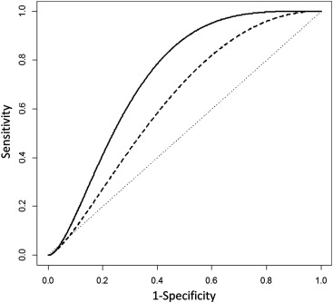
While these mean and covariance estimates are informative on their own, we substitute them into Equation 3 and get the BLC β→ˆT0=(0.164,−1.496,1.598) β

→

(

0.164

−

1.496

1.598

) . We could now apply these coefficients and generate a parametric ROC curve for the BLC, which we compare to a similar curve for PCB 180 in Figure 3 . It is obvious in Figure 3 that the estimated BLC ROC curve (solid) is completely and substantially higher than that of estimated PCB 180 (dashed) and implies a potential increase in discrimination. We can quantify this using the AUˆC0 A

0 by simply using Equation 4 to see what might be achieved using all three biomarkers jointly for separating women with and without endometriosis. Combining PCBs 188, 153, and 180 in this manner yields AUˆC0=0.731 A

0.731 , an increase in estimated discriminatory ability from any single biomarker. Using Equations A2 and A5 , we can also generate a 95% CI of 0.677 to 0.779. While these estimates show a potential benefit of using three biomarkers over one, ROC analysis is a process in which superiority of one biomarker over another for practical purposes needs to be validated with independent data before a recommendation can be made.

Get Radiology Tree app to read full this article<

Discussion

Get Radiology Tree app to read full this article<

Acknowledgments

Get Radiology Tree app to read full this article<

Appendix

Multivariate Normal Likelihood with Left Censoring

Get Radiology Tree app to read full this article<

g(W−→;μ→,Σ)=1(2π)p/2|Σ|1/2exp{−12(W−→−μ→)TΣ−1(W−→−μ→)}, g

(

→

;

→

)

(

)

exp

{

−

(

→

−

→

)

−

(

→

−

→

)

}

where the covariance matrix ∑ ∑ consists of variance, ∑ll=σll ∑

l , and covariance terms, Σll′=σll′ Σ

′

′ , l≠l′ l

≠

′ . Again, suppose that biomarker measurements Z→ Z

→ are observed. The first part necessary for creating a likelihood function for a sample matrix Z with which we can estimate μ→ μ

→ and ∑ ∑ is for those Z→ Z

→ with Q→(Z→)=(1,1,1,…,1) Q

→

(

→

)

(

…

) , where the likelihood function is the standard result L(μ→,Σ;Z→)=L1(μ→,Σ;w1,w2…,wp)=g(w→;μ→,Σ) L

(

→

;

→

)

(

→

;

…

)

(

→

;

→

) . Second, we skip to the other extreme for those Z→ Z

→ with Q→(Z→)=(0,0,0,…,0) Q

→

(

→

)

(

…

) , where the likelihood function corresponds to the probability

L(μ→,Σ;Z→)=L2p(μ→,Σ;w1<d1,w2<d2,…,wp<dp)=∫−∞d1∫−∞d2⋯∫−∞dpg(w→;μ→,Σ)dwp⋯dw2dw1=Λ(d→;μ→,Σ) L

(

→

;

→

)

(

→

;

…

)

∫

−

∞

∫

−

∞

⋯

∫

−

∞

(

→

;

→

)

⋯

(

→

;

→

)

Henceforth, Λ(d→;μ→,Σ) Λ

(

→

;

→

) will denote the probability that all of an individual’s biomarker levels are below the LODs for a given μ→ μ

→ and ∑ ∑ . For the likelihoods of all the cases of Q→(Z→) Q

→

(

→

) in between, Lk(μ→,Σ;Z→) L

(

→

;

→

) , k = 2,3, … , 2 p – 1 (ie, those Z→ Z

→ composed of both quantified and censored levels), we will extend ideas from explicit results for P = 2 to the general p case here . In that work, the bivariate normal case with Q→(Z→)=(1,0) Q

→

(

→

)

(

) or (0,1) was shown to lead to a likelihood that is the product of a marginal distribution for the biomarker that is observed and a conditional distribution for the biomarker measured below the LOD. We will rely on the same rationale here but allow the observed and unobserved to be vectors of biomarkers with marginal and conditional distributions that can themselves be multivariate.

Get Radiology Tree app to read full this article<

CZ→=⎡⎣⎢⎢⎢⎢⎢⎢0001010000010000000100100⎤⎦⎥⎥⎥⎥⎥⎥⎛⎝⎜⎜⎜⎜⎜⎜.w2w3.w5⎞⎠⎟⎟⎟⎟⎟⎟=⎛⎝⎜⎜⎜⎜⎜⎜w2w3w5..⎞⎠⎟⎟⎟⎟⎟⎟=⎛⎝⎜Z→(1)Z→(2)⎞⎠⎟ C

→

[

]

(

)

(

)

(

→

(

)

→

(

)

A consequence of this reordering is that CZ→∼Np(Cμ→,CΣCT) C

→

∼

(

→

) and that Cμ→=(μ→(1),μ→(2))T C

→

(

→

(

)

→

(

)

T and CΣCT=[Σ11Σ21Σ12Σ22] C

[

] can be similarly partitioned, where Σab Σ

ab can be a matrix, vector, or scalar depending on the partition. The resultant multivariate normal density is then factored into a marginal density, g(1)(W−→(1);μ→(1),Σ11) g

(

)

(

→

(

)

;

→

(

)

) , and a conditional density, g(2|1)(W−→(2);μ→(Q),ΣQ) g

(

)

(

→

(

)

;

→

(

)

) , with μ→(Q)=μ→(2)+Σ21Σ−111(W−→(1)−μ→(1)) μ

→

(

)

→

(

)

−

(

→

(

)

−

→

(

)

) and ΣQ=Σ22−Σ21Σ−111Σ12 Σ

−

12 . Since the observations in Z→(2) Z

→

(

) are unobserved but below the LODs, the likelihood for the k th unique Q→(Z→) Q

→

(

→

) , k = 2,3, … , 2 p – 1 is

Lk(μ→,Σ;Z→(1),Z→(2))∝g(1)(w→(1);μ→(1),Σ11)×∫−∞d→(2)g(2|1)(w→(2);μ→(Q),ΣQ)dw→(2)=g(1)(w→(1);μ→(1),Σ11)×Λ(2|1)(d→(2);μ→(Q),ΣQ) L

(

→

;

→

(

)

→

(

)

∝

(

)

(

→

(

)

;

→

(

)

∫

−

∞

→

(

)

(

)

(

→

(

)

;

→

(

)

→

(

)

(

)

(

→

(

)

;

→

(

)

(

)

(

→

(

)

;

→

(

)

Therefore, for a random sample Z of independent identically distributed p -dimensional vectors Z→j Z

→

j , j = 1, … , n , following a multivariate normal distribution, the likelihood has the form

(

→

;

)

∏

(

→

;

→

)

∝

∏

→

(

→

)

(

…

)

(

→

;

→

)

⋯

∏

→

(

→

)

(

…

)

(

)

(

→

(

)

;

→

(

)

(

)

(

→

(

)

;

→

(

)

⋯

∏

→

(

→

)

(

…

)

(

→

;

→

)

Maximizing Equation A1 with respect to each element of μ→ μ

→ and Σ Σ results in MLEs μ→ˆ μ

→

ˆ and Σˆ Σ

ˆ . This must be performed numerically due to the complexity of the likelihood for which a closed form solution does not exist for even the univariate case. Also of note is that for the explicit P = 2 case, Equation A1 reduces to the likelihood of Lyles et al . However, out of necessity, we maintain matrix notation rather than the explicit expansion displayed there.

Get Radiology Tree app to read full this article<

Fisher Information Matrix

Get Radiology Tree app to read full this article<

Cov(θ→ˆ)=Cov(μ→ˆ,Σˆ)=[I]−1=⎡⎣⎢⎢⎢I1,1⋮Ip(p+1),1⋯⋱⋯I1,p(p+1)⋮Ip(p+1),p(p+1)⎤⎦⎥⎥⎥, C

(

→

)

(

→

)

[

]

−

[

⋯

(

)

⋮

⋱

⋮

(

)

⋯

(

)

(

)

]

where ( P ≥ 2) and each Iab=limn→∞−1nE⎡⎣⎢∂2log(L(θ→;z→)∂θa∂θb⎤⎦⎥ I

lim

→

∞

−

[

∂

log

(

→

;

→

)

∂

] . Please note that the rows and columns of Equation A2 correspond to θ→=(μ→,Σ)T=(μ1,…,μp,σ11,σ12,…,σpp)T θ

→

(

→

)

(

…

)

T , a vector where the elements of Σ are listed out as a vector and concatenated with μ→ μ

→ . The development of the I__ab , based on the partial derivatives of the log likelihood in Equation A1 , was done with respect to the subvectors and matrices in μ→=(μ→(1),μ→(2))T μ

→

(

→

(

)

→

(

)

T and Σ=[Σ11Σ21Σ12Σ22] Σ

[

] in order to facilitate for the general p dimensionality of our data. The expected values of elements I__ab are explicitly evaluated where possible and are approximated otherwise.

Get Radiology Tree app to read full this article<

Estimated AUC for a BLC with CI

Get Radiology Tree app to read full this article<

β→T0∝(μ→X−μ→Y)T(ΣX+ΣY)(−1), β

→

∝

(

→

−

→

)

(

)

(

−

)

leading to

AUC0=P(U>V)=Φ((μ→X−μ→Y)T(ΣX+ΣY)−1(μ⇀X−μ⇀Y)−−−−−−−−−−−−−−−−−−−−−−−−−−−−−−−−√), A

(

)

(

→

−

→

)

(

)

−

(

⇀

−

⇀

)

which is “best” with respect to maximizing AUC over all real β→T β

→

T .

Get Radiology Tree app to read full this article<

σ2δ=λ−1(∂δ∂θ→X)T(Cov(θ→Xˆ))(∂δ∂θ→X)+(1−λ)−1(∂δ∂θ→Y)T(Cov(θ→Yˆ))(∂δ∂θ→Y), σ

−

(

∂

→

)

(

→

)

(

∂

→

)

(

−

)

−

(

∂

→

)

(

→

)

(

∂

→

)

with θ→=(μ→,Σ)T θ

→

(

→

)

T have the form described in Materials and Methods, and (∂δ∂θ→)ij=∂δ∂θ→ij (

∂

→

)

∂

→

j being the ij__th element of (∂δ∂θ→) (

∂

→

) , the partial derivative of δ with respect to the vectorized parameters. A 1 – α level CI for AUˆC0 A

0 can subsequently be calculated by Φ(δˆ±zα/2σ2δ√N√) Φ

(

) . Given μ→ˆX,μ→ˆY,ΣˆX μ

→

X , and ΣˆY Σ

Y based on Zx and ZY , we use this technique to calculate an approximately 1 – α level CI for AUˆC0 A

0 .

Get Radiology Tree app to read full this article<

References

1. Metz C.E.: Basic principles of ROC analysis. Semin Nucl Med 1978; 8: pp. 283-298.
2. Wagner R.F., Beiden S.V., Metz C.E.: Continuous versus categorical data for ROC analysis: some quantitative considerations. Acad Radiol 2001; 8: pp. 328-334.
3. Pepe M.S.: The statistical evaluation of medical tests for classification and prediction.2003.Oxford University PressNew York
4. Zhou X.H., Obuchowski N.A., McClish D.K.: Statistical methods in diagnostic medicine.2002.Wiley & Sons InterscienceNew York
5. Browne R.W., Whitcomb B.W.: Procedures for determination of detection limits: application to high-performance liquid chromatography analysis of fat-soluble vitamins in human serum. Epidemiology 2010; 21: pp. S4-S9.
6. Hornung R.W., Reed L.D.: Estimation of average concentration in the presence of nondetectable values. Appl Occup Environ Hyg 1990; 5: pp. 46-51.
7. Haas C.H., Scheff P.A.: Estimation of averages in truncated samples. Environ Sci Technol 1990; 24: pp. 912-919.
8. Lyles R.H., Williams J.K., Chuachoowong R.: Correlating two viral load assays with known detection limits. Biometrics 2001; 57: pp. 1238-1244.
9. Schisterman E.F., Little R.J.: Opening the black box of biomarker measurement error. Epidemiology 2010; 21: pp. S1-S3.
10. Singh A., Nocerino J.: Robust estimation of mean and variance using environmental data sets with below detection limit observations. Chemometr Intelligent Lab Syst 2002; 60: pp. 69-86.
11. Perkins N.J., Schisterman E.F., Vexler A.: Receiver operating characteristic curve inference from a sample with a limit of detection. Am J Epidemiol 2007; 165: pp. 325-333.
12. Gupta A.K.: Estimation of the mean and standard deviation of a normal population from a censored sample. Biometrika 1952; 39: pp. 260-273.
13. Harter H.L., Moore A.H.: Asymptotic variances and covariances of maximum-likelihood estimators, from censored samples, of the parameters of Weibull and gamma populations. Ann Math Stat 1967; 38: pp. 557-570.
14. Vexler A., Liu A., Eliseeva E., et. al.: Maximum likelihood ratio tests for comparing the discriminatory ability of biomarkers subject to limit of detection. Biometrics 2008; 64: pp. 895-903.
15. Perkins N.J., Schisterman E.F., Vexler A.: ROC curve inference for best linear combination of two biomarkers subject to limits of detection. Biometr J 2011; 53: pp. 464-476.
16. Su J.Q., Liu J.S.: Linear combinations of multiple diagnostic markers. J Am Stat Assoc 1993; 88: pp. 1350-1355.
17. Reiser B., Faraggi D.: Confidence intervales for the generalized ROC criterion. Biometrics 1997; 53: pp. 192-202.
18. Louis G., Weiner J.M., Whitcomb B.W., et. al.: Environmental PCB exposure and risk of endometriosis. Hum Reprod 2005; 20: pp. 279-285.
19. Cooke P.S., Sato T., Buchanan D.L.: Disruption of steroid hormone signaling by PCBs.Robertson L.W.Hansen L.G.PCBs: recent advances in environmental toxicology and health effects.2001.The University Press of KentuckyLexington:pp. 257-263.
20. Molodianovitch K., Faraggi D., Reiser B.: Comparing the areas under two correlated ROC curves: parametric and non-parametric approaches. Biometr J 2006; 48: pp. 745-757.
21. Pesce L.L., Metz C.E., Berbaum K.S.: On the convexity of ROC curves estimated from radiological test results. Acad Radiol 2010; 17: pp. 960-968.
22. Pesce L.L., Horsch K., Drukker K., et. al.: Semiparametric estimation of the relationship between ROC operating points and the test-result scale: application to the proper binormal model. Acad Radiol 2011; 18: pp. 1537-1548.
23. Samuelson F., Gallas B.D., Myers K.J., et. al.: The importance of ROC data. Acad Radiol 2011; 18: pp. 257-258. author reply 259–261
24. Alemayehu D., Zou K.H.: Applications of ROC analysis in medical research: recent developments and future directions. Acad Radiol 2012; 19: pp. 1457-1464.
25. Hillis S.L., Metz C.E.: An analytic expression for the binormal partial area under the ROC curve. Acad Radiol 2012; 19: pp. 1491-1498.

Multivariate Normally Distributed Biomarkers Subject to Limits of Detection and Receiver Operating Characteristic Curve Inference

Rationale and Objectives

Materials and Methods

Results

Conclusions

Materials and methods

Left-Censored Multivariate Normal Likelihood

ROC Curve and the AUC

Results

Example

Discussion

Acknowledgments

Appendix

Multivariate Normal Likelihood with Left Censoring

Fisher Information Matrix

Estimated AUC for a BLC with CI

References

Further Reading

A Brief History of Free-Response Receiver Operating Characteristic Paradigm Data Analysis

An Additive Selection of Markers to Improve Diagnostic Accuracy Based on a Discriminatory Measure

An Examination of Data Confidentiality and Disclosure Issues Related to Publication of Empirical ROC Curves