
Rationale and Objectives
The aims of this study were to propose a semiautomated technique to segment and measure the volume of different nerve components of the tibial nerve, such as the nerve fascicles and the epineurium, based on magnetic resonance microneurography and a segmentation tool derived from brain imaging; and to assess the reliability of this method by measuring interobserver and intraobserver agreement.
Materials and Methods
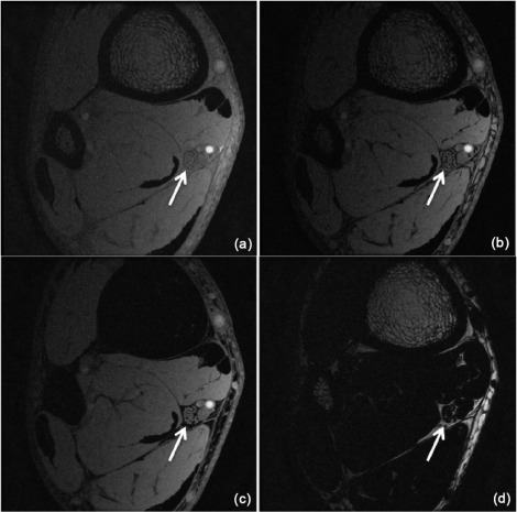
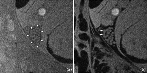
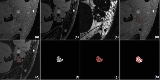
The tibial nerve of 20 healthy volunteers (age range = 23–69; mean = 47; standard deviation = 15) was investigated at the ankle level. High-resolution images were obtained through tailored microneurographic sequences, covering 28 mm of nerve length. Two operators manually segmented the nerve using the in-phase image. This region of interest was used to mask the nerve in the water image, and two-class segmentation was performed to measure the fascicular volume, epineurial volume, nerve volume, and fascicular to nerve volume ratio (FNR). Interobserver and intraobserver agreements were calculated.
Results
The nerve structure was clearly visualized with distinction of the fascicles and the epineurium. Segmentation provided absolute volumes for nerve volume, fascicular volume, and epineurial volume. The mean FNR resulted in 0.69 with a standard deviation of 0.04 and appeared to be not correlated with age and sex. Interobserver and intraobserver agreements were excellent with alpha values >0.9 for each parameter investigated, with measurements free of systematic errors at the Bland-Altman analysis.
Conclusions
We concluded that the method is reproducible and the parameter FNR is a novel feature that may help in the diagnosis of neuropathies detecting changes in volume of the fascicles or the epineurium.
Introduction
Peripheral nerve pathology reflects in a variety of histopathologic patterns. The Seddon classification is traditionally used to divide acute nerve injuries into neuroapraxia (axonal strain with temporary functional loss), axonotmesis (axonal cut short with Wallerian degeneration), and neurotmesis (discontinuity also of the supporting connective tissues) . Chronic neuropathies are associated with additional modifications such as collagen deposition on the extracellular matrix, basement membrane thickening and changes in volume of the connective sheaths (ie, the epi-, peri- and endoneurium), nerve fibers loss, demyelination, remyelination, and Schwann cell proliferation .
The assessment of peripheral nerve disorders is achieved through medical history and physical examination, supported by instrumental investigations including electrophysiology, nerve biopsy, and magnetic resonance imaging (MRI). Electrophysiology detects gross distribution of nerve dysfunction, but it is limited for determining the exact location of nerve injury and cannot depict morphological alterations within the nerve . Histopathology may be carried out in vivo with the biopsy of the sural nerve, which can be sacrificed in restricted circumstances. Furthermore, the sural nerve contains only sensitive fibers and the specimens may not necessarily represent the underlying disease . MRI is the most advanced imaging technique available for the study of peripheral nerves, with the advantages to be noninvasive and repeatable . Standard protocols for MRI of peripheral nerves, also known as magnetic resonance (MR) neurography , include high-resolution axial T1-weighted and fat-suppressed T2-weighted images . As injured nerves appear hyperintense on T2-weighted images, several studies have focused on the increased T2 relaxation time to evaluate the nerve damage . However, the morphological detail usually achieved is insufficient for visualization of the single nerve fascicles and the tissues within and around.
Get Radiology Tree app to read full this article<
Get Radiology Tree app to read full this article<
Get Radiology Tree app to read full this article<
Materials and Methods
Subjects
Get Radiology Tree app to read full this article<
Table 1
Mean Age with Standard Deviation (SD) of the Subjects Included in the Study Divided by Gender
Gender Subjects Age Mean SD Males 13 42.9 14.8 Females 7 50.3 13.8 Total 20 45.3 14.6
Get Radiology Tree app to read full this article<
Imaging Protocol
Get Radiology Tree app to read full this article<
Get Radiology Tree app to read full this article<
Image Processing and Segmentation
Get Radiology Tree app to read full this article<
Get Radiology Tree app to read full this article<
Statistical Analysis
Get Radiology Tree app to read full this article<
Results
Get Radiology Tree app to read full this article<
Get Radiology Tree app to read full this article<
Table 2
Intraobserver and Interobserver Agreements Investigated with the Intraclass Correlation Coefficient for Absolute Agreement ICC
Mean (mm 3 ) SD α Intraobserver agreement Nerve volume First measurement 252.58 52.92 0.970 Second measurement 259.90 47.01 Interobserver agreement Nerve volume First operator 292.84 61.41 0.983 Second operator 288.17 57.95 Fascicles volume First operator 201.76 38.55 0.987 Second operator 198.52 34.54 Fascicles to nerve ratio (FNR) First operator 0.693 0.042 0.986 Second operator 0.694 0.045
All alpha coefficients for the parameters investigated are > 0.9 consistent with very high agreement. SD, standard deviation.
Get Radiology Tree app to read full this article<
Get Radiology Tree app to read full this article<
Table 3
Reliability of the Measurements between the Two Examiners using Bland-Altman Analysis
Mean Difference Confidence Interval p 5% 95% Nerve volume 2.565 −21.710 26.840 0.366 Fascicles volume 1.785 −15.365 18.935 0.373 FNR −0.001 −0.020 0.018 0.635 Epineurial volume 0.660 −8.890 10.210 0.552
Mean differences are reported with the limits of agreement graphically represented in Table 5 . There is no statistical difference between the measurements of the two operators for NV, FV, EV and FNR (p > 0.05) and no systematic errors on the measurements. EV, epineurial volume; FNR, fascicular to nerve volume ratio; FV, fascicular volume; NV, nerve volume.
Table 4
Bland-Altman plots for NV, FV, EV, and FNR.
Open full size image
In these scatter plots, the Y axis represents the differences of the two measurements, which are plotted against their mean represented on the Y axis. The central horizontal line represents the mean difference of the two examiners, and the upper and lower lines represent their agreement limits, in which at least 95% of the data points lie. All confidence interval limits of the mean include the zero line, thus no statistically significant bias is present between the measurements. EV, epineurial volume; FNR, fascicular to nerve volume ratio; FV, fascicular volume; NV, nerve volume.
Table 5
Pearson Correlation Coefficients
NV FV FNR EV Age Pearson correlation 0.458 0.423 −0.199 0.441 Sig. (2-code) 0.037 0.056 0.386 0.045 Gender Pearson correlation 0.113 0.078 −0.145 0.149 Sig. (2-code) 0.626 0.738 0.529 0.519
There is statistical positive correlation between age and NV, EV (p < 0.05), and borderline correlation with FV (p = 0.056). There is no correlation between age and FNR and between sex and any of the parameters investigated. EV, epineurial volume; FNR, fascicular to nerve volume ratio; FV, fascicular volume; NV, nerve volume.
Get Radiology Tree app to read full this article<
Discussion
Get Radiology Tree app to read full this article<
Get Radiology Tree app to read full this article<
Get Radiology Tree app to read full this article<
Get Radiology Tree app to read full this article<
Get Radiology Tree app to read full this article<
Get Radiology Tree app to read full this article<
Get Radiology Tree app to read full this article<
Get Radiology Tree app to read full this article<
References
1. Aagaard B.D., Lazar D.A., Lankerovich L., et. al.: High-resolution magnetic resonance imaging is a noninvasive method of observing injury and recovery in the peripheral nervous system. Neurosurgery 2003; 53: pp. 199-203. discussion 03-4
2. Anghinah A., Bastos de Jorge F., Aisen J.: Chemical composition of peripheral nerves. Clin Chem 1969; 15: pp. 1230-1233.
3. Baumer P., Weiler M., Bendszus M., et. al.: Somatotopic fascicular organization of the human sciatic nerve demonstrated by MR neurography. Neurology 2015; 84: pp. 1782-1787.
4. Bilgen M., Heddings A., Al-Hafez B., et. al.: Microneurography of human median nerve. J Magn Reson Imaging 2005; 21: pp. 826-830.
5. Bydder G.M., Znamirowski R.M., Carl M., et. al.: MR imaging of peripheral nerves with short and ultrashort echo pulse sequences.21st annual scientific meeting of international society of magnetic resonance in medicine.2013. Salt Lake City, UT
6. Chalian M., Faridian-Aragh N., Soldatos T., et. al.: High-resolution 3T MR neurography of suprascapular neuropathy. Acad Radiol 2011; 18: pp. 1049-1059.
7. Chhabra A.: Magnetic resonance neurography—simple guide to performance and interpretation. Semin Roentgenol 2013; 48: pp. 111-125.
8. Chhabra A., Belzberg A.J., Rosson G.D., et. al.: Impact of high resolution 3 Tesla MR neurography (MRN) on diagnostic thinking and therapeutic patient management. Eur Radiol 2016; 26: pp. 1235-1244.
9. Conversano F., Franchini R., Demitri C., et. al.: Hepatic vessel segmentation for 3D planning of liver surgery experimental evaluation of a new fully automatic algorithm. Acad Radiol 2011; 18: pp. 461-470.
10. Eggert L.D., Sommer J., Jansen A., et. al.: Accuracy and reliability of automated gray matter segmentation pathways on real and simulated structural magnetic resonance images of the human brain. PLoS ONE 2012; 7: pp. e45081.
11. Felisaz P.F., Chang E.Y., Carne I., et. al.: In vivo MR microneurography of the tibial and common peroneal nerves. Radiol Res Pract 2014; 2014: pp. 780964.
12. Filler A.G., Howe F.A., Hayes C.E., et. al.: Magnetic resonance neurography. Lancet 1993; 341: pp. 659-661.
13. Filler A.G., Kliot M., Howe F.A., et. al.: Application of magnetic resonance neurography in the evaluation of patients with peripheral nerve pathology. J Neurosurg 1996; 85: pp. 299-309.
14. Fuller S., Reeder S., Shimakawa A., et. al.: Iterative decomposition of water and fat with echo asymmetry and least-squares estimation (ideal) fast spin-echo imaging of the ankle: initial clinical experience. AJR Am J Roentgenol 2006; 187: pp. 1442-1447.
15. Gerdes C.M., Kijowski R., Reeder S.B.: Ideal imaging of the musculoskeletal system: robust water fat separation for uniform fat suppression, marrow evaluation, and cartilage imaging. AJR Am J Roentgenol 2007; 189: pp. W284-W291.
16. Grant G.A., Britz G.W., Goodkin R., et. al.: The utility of magnetic resonance imaging in evaluating peripheral nerve disorders. Muscle Nerve 2002; 25: pp. 314-331.
17. Heddings A., Bilgen M., Nudo R., et. al.: High-resolution magnetic resonance imaging of the human median nerve. Neurorehabil Neural Repair 2004; 18: pp. 80-87.
18. Ikeda K., Haughton V.M., Ho K.C., et. al.: Correlative MR—anatomic study of the median nerve. AJR Am J Roentgenol 1996; 167: pp. 1233-1236.
19. Klauschen F., Goldman A., Barra V., et. al.: Evaluation of automated brain MR image segmentation and volumetry methods. Hum Brain Mapp 2009; 30: pp. 1310-1327.
20. Kollmer J., Bendszus M., Pham M.: MR neurography: diagnostic imaging in the PNS. Clin Neuroradiol 2015; 25: pp. 283-289.
21. Kollmer J., Hund E., Hornung B., et. al.: In vivo detection of nerve injury in familial amyloid polyneuropathy by magnetic resonance neurography. Brain 2014; 138: pp. 549-562.
22. Kundalic B., Ugrenovic S., Jovanovic I., et. al.: Morphometric analysis of connective tissue sheaths of sural nerve in diabetic and nondiabetic patients. Biomed Res Int 2014; 2014: pp. 870930.
23. Kwee R.M., Chhabra A., Wang K.C., et. al.: Accuracy of MRI in diagnosing peripheral nerve disease: a systematic review of the literature. AJR Am J Roentgenol 2014; 203: pp. 1303-1309.
24. Lundborg G.: Nerve injury and repair: regeneration, reconstruction, and cortical remodeling.2004.Elsevier/Churchill Livingstone.Philadelphia, PA
25. Pham M., Baumer P., Meinck H.M., et. al.: Anterior interosseous nerve syndrome: fascicular motor lesions of median nerve trunk. Neurology 2014; 82: pp. 598-606.
26. Pham M., Oikonomou D., Baumer P., et. al.: Proximal neuropathic lesions in distal symmetric diabetic polyneuropathy: findings of high-resolution magnetic resonance neurography. Diabetes Care 2011; 34: pp. 721-723.
27. Reeder S.B., McKenzie C.A., Pineda A.R., et. al.: Water-fat separation with ideal gradient-echo imaging. J Magn Reson Imaging 2007; 25: pp. 644-652.
28. Seddon H.J., Medawar P.B., Smith H.: Rate of regeneration of peripheral nerves in man. J Physiol 1943; 102: pp. 191-215.
29. Stoll G., Bendszus M., Perez J., et. al.: Magnetic resonance imaging of the peripheral nervous system. J Neurol 2009; 256: pp. 1043-1051.
30. Sunderland Sir S.: Nerves and nerve injuries.1978.Churchill LivingstoneEdimburgh (UK); New York (NY):
31. Thakkar R.S., Del Grande F., Thawait G.K., et. al.: Spectrum of high-resolution MRI findings in diabetic neuropathy. AJR Am J Roentgenol 2012; 199: pp. 407-412.
32. Ushiki T., Ide C.: Three-dimensional organization of the collagen fibrils in the rat sciatic nerve as revealed by transmission-and scanning electron microscopy. Cell Tissue Res 1990; 260: pp. 175-184.
33. Zhang Y., Brady M., Smith S.: Segmentation of brain MR images through a hidden Markov random field model and the expectation-maximization algorithm. IEEE Trans Med Imaging 2001; 20: pp. 45-57.