Nonrigid Registration for Subtraction CT Angiography Applied to the Carotids and Cranial Art eries

Rationale and Objectives

Computed tomography angiography (CTA) is an established tool for vascular imaging. However, high-intensity nonvascular structures in the contrast image can seriously hamper luminal visualization. This is an issue for three-dimensional visualization, where high-intensity structures might cover the underlying vasculature. But also in two dimensions, calcified plaques adjacent to the contrast-enhanced vessel lumen impede correct determination of the vessel boundary. High-intensity structures can be eliminated using subtraction CTA, where a native image is subtracted from the contrast image. However, patient and organ motion limits the widespread application of this technique. We propose to use nonrigid image registration to solve this problem.

Materials and Methods

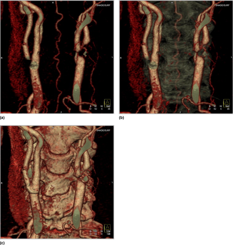
For each patient, a native image and a contrast image are recorded, respectively, before and after contrast administration. The native image is registered to the contrast image using an automatic intensity-based nonrigid three-dimensional registration algorithm. Both images are merged in a fused image, allowing the user to switch between a view of the arteries, the bone or both. The procedure has been applied to 95 patients.

Results

In all cases, subtraction CTA using nonrigid registration allows for a significantly better artifacts removal than subtraction CTA without registration. Image quality of all images was judged adequate for clinical use. The average total processing time for each dataset is about 30 minutes.

Conclusion

Nonrigid registration can allow for a great reduction in subtraction artifacts for subtraction CTA, resulting in a clear view of the vasculature.

Computed tomography (CT) angiography (CTA) is an established minimally invasive tool for imaging major and minor vessels in the body ( ). Since the introduction of CTA more than 10 years ago, ongoing development of CT modalities resulted in shorter image acquisition time, improved volume coverage, and a better spatial resolution. With current 16-, 64-, or even 256-channel multidetector CT scanners, the temporal resolution has increased sufficiently to enable cardiac synchronization. The increased spatial resolution allows a detailed view of not only the main vessels but also ever smaller vessels.

However, these new scanning techniques also create an increasing amount of data, requiring a change in the way CTA studies are visualized and interpreted. In a traditional CTA examination, the radiologist will scroll through the different coronal, axial and transversal two-dimensional (2D) slices, using slice distances of 1 to 5 mm. This procedure is time consuming, and barely benefits from the improved spatial resolution of current CT modalities.

Get Radiology Tree app to read full this article<

Materials and methods

Get Radiology Tree app to read full this article<

To get an optimal result, it is necessary to control each step in the image processing chain, from acquisition to visualization. In the following paragraphs we will provide more details on steps 1, 2, 4, 5, and 7. For the data transmission in steps 3 and 6, Digital Imaging and Communications in Medicine (ie, DICOM) protocol is used.

Get Radiology Tree app to read full this article<

Recording Setup

Get Radiology Tree app to read full this article<

Image Registration

Get Radiology Tree app to read full this article<

Transformation Model

Get Radiology Tree app to read full this article<

g→(r→;μ)=∑ijkμijk⋅β2Δx(x−kxi)⋅β2Δy(y−kyj)⋅β2Δz(z−kzk), g

→

(

→

;

)

∑

⋅

(

−

)

⋅

(

−

)

⋅

(

−

)

with βnε(x)=ε−1βn(x/ε) β

(

)

−

(

) the expanded B-spline of degree n n and kξ=Δξ(−1/2) k

(

−

) (for ι=i,j,k ι

k , respectively ξ=x,y,z ξ

z ).

Get Radiology Tree app to read full this article<

Similarity Measure

Get Radiology Tree app to read full this article<

∀r∈BR,f∈BF:p(r,f;μ)=∑r→∈(R∩F’)w(f−IF(g→(r→;μ))εf)w(r−IR(r→)εr) ∀

∈

(

;

)

∑

→

∈

(

∩

′

)

(

−

(

→

(

→

;

)

(

−

(

→

)

p(f;μ)=∑r∈BRp(r,f;μ), p

(

;

)

∑

∈

(

;

)

p(r)=∑f∈BFp(r,f;μ) p

(

)

∑

∈

(

;

)

with B f and B r being the number of bins. For the window function w(x) = β 2 ( x ), the second-degree B-spline was used.

Get Radiology Tree app to read full this article<

I(R,F;Φ)=∑r∈BR∑f∈BFp(r,f;Φ)log(p(r,f;Φ)p(r)⋅p(f;Φ)) I

(

;

)

∑

∈

∑

∈

(

;

)

log

⁡

(

;

)

(

)

⋅

(

;

)

is calculated, which is used as similarity measure.

Get Radiology Tree app to read full this article<

Multiresolution Scheme

Get Radiology Tree app to read full this article<

Image Fusion

Get Radiology Tree app to read full this article<

Iv={ϑs,Ic−In+ϑs,(Ic<ϑs)∨(Ic<In)∨(In<ϑa)otherwise. I

{

(

)

∨

(

)

∨

(

)

−

otherwise

Thus all voxels in I v have an intensity greater than ϑs ϑ

s . Next the bone image is created as the difference between the contrast and the vessel image:

Ib={Ic−Iv+ϑs,ϑs,Ic≥Iv;Ic<Iv. I

{

−

≥

;

Finally, the fused image I f is created, in which soft-tissue voxels are set to ϑs, ϑ

, vessel intensities remain unchanged, and bone voxel intensities are mirrored around ϑs: ϑ

If={Iv,2ϑs−min(Ib,2ϑs),Ib−Iv≤ϑd;Ib−Iv>ϑd, I

{

−

≤

;

−

min

⁡

(

)

−

This leads to a fused image histogram in which the vessel voxel intensities remain situated in the range around 300 HU, all soft tissue is concentrated at ϑs ϑ

s and the bone voxel intensities are situated in the range [−1024, ϑ s − ϑ d ]. Therefore vessel and bone intensities are well separated in the histogram. An example of a fused image histogram is presented in Fig 1 .

Get Radiology Tree app to read full this article<

Visualization

Get Radiology Tree app to read full this article<

Validation Measure

Get Radiology Tree app to read full this article<

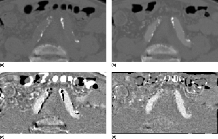
Table 1

Overview of the Intensity Differences Between the Structures of Interest in Subtraction CT Images (in Hounsfield Units)

Contrast Soft Tissue Vessel Plaque Native ∼0 ∼400 >400 Soft tissue ∼0 ∼0 ∼400 >400 Vessel ∼0 ∼0 ∼400 >400 Plaque >400 ≤400 <0 ∼0

Get Radiology Tree app to read full this article<

Q=In(r→)−Iv(r→)¯¯¯¯¯¯¯¯¯¯¯¯¯¯¯¯¯¯¯¯¯¯¯¯¯,∀r→:In(r→)>Iv(r→). Q

(

→

)

−

(

→

)

∀

→

(

→

)

(

→

)

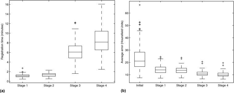
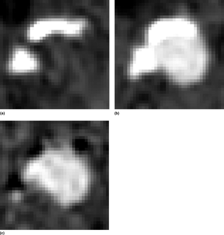
To visually assess the registration quality, error images are created showing the sum of the negative voxels in the difference images. Darker pixels reflect more artifacts and thus a worse registration; bright pixels indicate no errors. The images give an indication of the location of the registration artifacts and a visual demonstration of the artifact reduction over increasing registration stages.

Get Radiology Tree app to read full this article<

Results

Get Radiology Tree app to read full this article<

$Figure 3, A box and whisker plot of (a) the registration time and (b) the average error per stage. Although only a fraction of the calculation time is spent in the first two stages, they provide the largest error reduction. However, the remaining stages are required to obtain clinically acceptable images. The boxes have lines at the lower quartile, median, and upper quartile values. The whiskers extend from each end of the box to show the extent of the rest of the data, whereas outliers are pictured individually.$

Get Radiology Tree app to read full this article<

Discussion

Get Radiology Tree app to read full this article<

Conclusions

Get Radiology Tree app to read full this article<

References

1. A Napoli A., Fleischmann D., Chan F.P., et. al.: Computed tomography angiography: state-of-the art imaging using multidetector-row technology. J Comput Assist Tomogr 2004; 28: pp. S32-S45.
2. Duddalwar V.A.: Multislice CT angiography: a practical guide to CT angiography in vascular imaging and intervention. Br J Radiol 2004; 77: pp. S27-S38.
3. Beier J., Oellinger H., Richter C.S., et. al.: Felix, registered image subtraction for CT-, MR- and coronary angiography. Eur Radiol 1997; 7: pp. 82-89.
4. Kwon S.M., Kim Y.S., Kim T.-S., et. al.: Digital subtraction CT angiography based on efficient 3D registration and refinement. Comput Med Imaging Graph 2004; 28: pp. 391-400.
5. Poletti P.-A., Rosset A., Didier D., et. al.: Subtraction CT angiography of the lower limbs: a new technique for the evaluation of acute arterial occlusion. AJR Am J Roentgenol 2004; 183: pp. 1445-1448.
6. van Straten M., Venema H.W., Streekstra G.J., et. al.: Removal of bone in CT angiography of the cervical arteries by piecewise matched mask bone elimination. Med Phys 2004; 31: pp. 2924-2933.
7. Rohlfing T., Maurer C.R., Beier J.: Reduction of motion artifacts in three-dimensional CT-DSA using constrained adaptive multilevel free-form registration. Comput Assisted Radiol Surg 2001; pp. 350-355.
8. Thévenaz P., Unser M.: Optimization of mutual information for multiresolution image registration. IEEE Trans Signal Proc 2008; 9: pp. 2083-2099.
9. Loeckx D.: Automated non-rigid intra-patient image registration using splines.2006. Ph.D. thesis, Katholieke Universiteit Leuven
10. American Hearth Association, American Stroke Association. Heart disease and stroke statistics—2004 update. Available online at http://www.americanhearth.org .
11. Bartlett E.S., Walters T.D., Symons S.P., et. al.: Quantification of carotid stenosis on CT angiography. AJNR Am J Neuroradiol 2006; 27: pp. 13-19.
12. Josephson S.A., Bryant S.O., Mak H.K., et. al.: Evaluation of carotid stenosis using CT angiography in the initial evaluation of stroke and TIA. Neurology 2004; 63: pp. 457-460.
13. Lell M., Anders K., Klotz E., et. al.: Clinical evaluation of bone-subtraction CT angiography (BSCTA) in head and neck imaging. Eur Radiol 2006; 16: pp. 889-897.
14. Sakamoto S., Kiura Y., Shibukawa M., et. al.: Subtracted 3D CT angiography for evaluation of internal carotid artery aneurysms: comparison with conventional digital subtraction angiography. AJNR Am J Neuroradiol 2006; 27: pp. 1332-1337.
15. McKinney A.M., Casey S.O., Teksam M., et. al.: Carotid bifurcation calcium and correlation with percent stenosis of the internal carotid artery on CT angiography. Neuroradiology 2005; 47: pp. 1-9.
16. Bub L.D., Hollingworth W., Jarvik J.G., et. al.: Screening for blunt cerebrovascular injury: Evaluating the accuracy of multidetector computed tomographic angiography. J Trauma 2005; 59: pp. 691-697.
17. Bash S., Villablanca J.P., Jahan R., et. al.: Intracranial vascular stenosis and occlusive disease: evaluation with CT angiography, MR angiography, and digital subtraction angiography. AJNR Am J Neuroradiol 2005; 26: pp. 1012-1021.
18. Kinoshita T., Ogawa T., Kado H., et. al.: CT angiography in the evaluation of intracranial occlusive disease with collateral circulation: comparison with MR angiography. Clin Imaging 2005; 29: pp. 303-306.
19. Sims J.R., Rordorf G., Smith E.E., et. al.: Arterial occlusion revealed by CT angiography predicts NIH stroke score and acute outcomes after IV tPA treatment. AJNR Am J Neuroradiol 2005; 26: pp. 246-251.
20. Tomandl B.F., Hammen T., Klotz E., et. al.: Bone subtraction CT angiography for the evaluation of intracranial aneurysms. AJNR Am J Neuroradiol 2006; 27: pp. 55-59.
21. Goddard A.J.P., Tan G., Becker J.: Computed tomography angiography for the detection and characterization of intra-cranial aneurysms: current status. Clin Radiol 2005; 60: pp. 1221-1236.
22. Kangasniemi M., Mäkelä T., Koskinen S., et. al.: Detection of intracranial aneurysms with two-dimensional and three-dimensional multislice helical computed tomographic angiography. Neurosurgery 2004; 54: pp. 336-340. discussion 340–341
23. Pechlivanis I., Schmieder K., Scholz M., König M., et. al.: 3-Dimensional computed tomographic angiography for use of surgery planning in patients with intracranial aneurysms. Acta Neurochir (Wien) 2005; 147: pp. 1045-1053.
24. Tipper G., U-King-Im J.M., Price S.J., et. al.: Detection and evaluation of intracranial aneurysms with 16-row multislice CT angiography. Clin Radiol 2005; 60: pp. 565-572.
25. van der Schaaf I., van Leeuwen M., Vlassenbroek A., et. al.: Minimizing clip artifacts in multi CT angiography of clipped patients. AJNR Am J Neuroradiol 2006; 27: pp. 60-66.
26. Papke K., Brassel F.: Modern cross-sectional imaging in the diagnosis and follow-up of intracranial aneurysms. Eur Radiol 2006; 16: pp. 2051-2066.
27. Coenen V.A., Dammert A., Reinges M.R.T., et. al.: Image-guided microneurosurgical management of small cerebral arteriovenous malformations: the value of navigated computed tomographic angiography. Neuroradiology 2005; 47: pp. 66-72.
28. Chen Z.K., Ning R.L.: Forest representation of vessels in cone-beam computed tomographic angiography. Comput Med Imaging Graph 2005; 29: pp. 1-14.
29. Suzuki Y., Nakajima M., Ikeda H., et. al.: Three-dimensional computed tomography angiography of the galenic system for the occipital transtentorial approach. Neurol Med Chir (Tokyo) 2005; 45: pp. 387-394.
30. Maes F., Collignon A., Vandermeulen D., et. al.: Multimodality image registration by maximization of mutual information. IEEE Trans Med Imaging 1997; 16: pp. 187-198.
31. Rueckert D., Sonoda L.I., Hayes C., et. al.: Nonrigid registration using free-form deformations: application to breast MR images. IEEE Trans Med Imaging 1999; 18: pp. 712-721.
32. Viola P., Wells W.M.: Alignment by maximization of mutual information. Int J Comp Vision 1997; 24: pp. 137-154.
33. Rohlfing T., Maurer C.R., Bluemke D.A., et. al.: Volume-preserving nonrigid registration of MR breast images using free-form deformation with an incompressibility constraint. IEEE Trans Med Imaging 2003; 22: pp. 730-741.
34. Loeckx D., Maes F., Vandermeulen D., et. al.: Temporal subtraction of thorax CR images using a statistical deformation model. IEEE Trans Med Imaging 2003; 22: pp. 1490-1504.
35. Loeckx D., Maes F., Vandermeulen D., et. al.: Comparison between Parzen window interpolation and generalised partial volume estimation for non-rigid image registration using mutual information. Workshop on Biomedical Image Registration, Lecture Notes in Computer Science 2006; pp. 206-213.
36. West J.J., Fitzpatrick J.M., Wang M.Y., et. al.: Comparison and evaluation of retrospective intermodality brain image registration techniques. J Comput Assist Tomogr 1997; 21: pp. 554-566.

Nonrigid Registration for Subtraction CT Angiography Applied to the Carotids and Cranial Art eries

Rationale and Objectives

Materials and Methods

Results

Conclusion

Materials and methods

Recording Setup

Image Registration

Transformation Model

Similarity Measure

Multiresolution Scheme

Image Fusion

Visualization

Validation Measure

Results

Discussion

Conclusions

References

Further Reading

Abstracts of Funded National Institutes of Health Grants (December)

Computer-Aided Diagnosis Scheme for Detection of Lacunar Infarcts on MR Images

Congresses, Conferences, Meetings, and Seminars