Novel Logistic Regression Model of Chest CT Attenuation Coefficient Distributions for the Automated Detection of Abnormal (Emphysema or ILD) Versus Normal Lung

Rationale and Objectives

We evaluated the role of automated quantitative computed tomography (CT) scan interpretation algorithm in detecting interstitial lung disease (ILD) and/or emphysema in a sample of elderly subjects with mild lung disease. We hypothesized that the quantification and distributions of CT attenuation values on lung CT, over a subset of Hounsfield units (HUs) range (−1000 HU, 0 HU), can differentiate early or mild disease from normal lung.

Materials and Methods

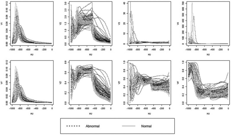
We compared the results of quantitative spiral rapid end-exhalation (functional residual capacity, FRC) and end-inhalation (total lung capacity, TLC) CT scan analyses of 52 subjects with radiographic evidence of mild fibrotic lung disease to the results of 17 normal subjects. Several CT value distributions were explored, including (1) that from the peripheral lung taken at TLC (with peels at 15 or 65 mm), (2) the ratio of (1) to that from the core of lung, and (3) the ratio of (2) to its FRC counterpart. We developed a fused-lasso logistic regression model that can automatically identify sub-intervals of −1000 HU and 0 HU over which a CT value distribution provides optimal discrimination between abnormal and normal scans.

Results

The fused-lasso logistic regression model based on (2) with 15-mm peel identified the relative frequency of CT values of over −1000 HU and −900 and those over −450 HU and −200 HU as a means of discriminating abnormal versus normal lung, resulting in a zero out-sample false-positive rate, and 15% false-negative rate of that was lowered to 12% by pooling information.

Conclusions

We demonstrated the potential usefulness of this novel quantitative imaging analysis method in discriminating ILD and/or emphysema from normal lungs.

Interstitial lung disease (ILD) is increasing in importance in part because of the aging population but also detection and/or incidence appear to be increasing. Data from the National Center for Health Statistics indicate that the age-adjusted mortality rate from pulmonary fibrosis has increased by 28.4% in men and by 41.3% in women between 1992 and 2014 .

Inter- and intrareader variability in the interpretation of radiographs for pulmonary fibrosis and pneumoconiosis has been long recognized as a potential issue for screening programs, epidemiologic studies, and medico-legal evaluations . Studies have found variable degrees of agreement for both parenchymal and pleural fibroses dependent on the extent of abnormalities and the training and medical specialty of the chest X-ray (CXR) readers . The National Institute for Occupational Safety and Health recommends using multiple, International Labour Organization radiographic pneumoconiosis classification system (ILO system)-trained readers and median profusion scores as the preferred reconciliation protocol to increase accuracy and precision in PA film classification . Clinical studies suggest that computed tomography (CT) imaging technology may become a gold standard for the evaluation of obstructive airways disease , but the literature is relatively limited on CT’s use in quantifying and objectively characterizing patterns of subtle interstitial fibrosis.

Get Radiology Tree app to read full this article<

Materials and Methods

Data

Get Radiology Tree app to read full this article<

Table 1

Demographic and Clinical Characteristics of Study Populations

ILD Normal_P_ Value_N_ 52 17 Sex 0.0002 Male 48 (92%) 8 (47%) Female 4 (8%) 9 (53%) Age, year 77.35 ± 8.41 40.35 ± 16.66 <0.0001 Race 0.16 African American 0 (0%) 1 (6%) Caucasian 50 (96%) 16 (94%) Hispanic 2 (4%) 0 (0%) BMI 28.81 ± 5.25 25.65 ± 3.69 0.025 Smoking history 0.00006 Never 20 (38%) 17 (100%) Former 25 (48%) 0 (0%) Current 7 (14%) 0 (0%) Pack-years 42.39 ± 34.47 0 ± 0 0.003 Plaques <0.0001 No 32 (62%) 17 (100%) Yes 20 (38%) 0 (0%) Emphysema <0.0001 No 6 (12%) 17 (100%) Yes 46 (88%) 0 (0%) Bronchiectasis <0.0001 No 9 (17%) 17 (100%) Yes 43 (83%) 0 (0%)

BMI, body mass index; ILD, interstitial lung disease.

Table 2

Pulmonary Function in Patients with ILD Compared to Normal Subjects

ILD Normal_P_ Value_N_ 52 17 TLC 96.41 ± 22.20 103.41 ± 8.52 0.21 RV 96.08 ± 31.26 100.18 ± 17.44 0.61 FVC 82.71 ± 24.11 109.76 ± 19.62 <0.0001 FEV 1 78.40 ± 24.40 112.82 ± 20.66 <0.0001 DLCO 62.25 ± 19.91 126.71 ± 15.81 <0.0001 FEV 1 /FVC 68.88 ± 14.14 82.94 ± 6.43 0.0002

DLCO, diffusion capacity for the lungs of carbon monoxide; FEV 1 , forced expiratory volume in 1 s; FVC, functional vital capacity; RV, residual volume; TLC, total lung capacity.

Get Radiology Tree app to read full this article<

Logistic Regression Model

Get Radiology Tree app to read full this article<

logit(p)=β0+∑Mj=1βjV(νj) logit

(

)

∑

(

)

where logit(p)=log{p/(1−p)} logit

(

)

log

{

(

−

)

} is the logistic transformation; p is the probability that the subject is abnormal, i.e. having lung disease; M is the total number of bins, here 100; ν j the center of the jth j

h bin; and β j = β ( ν j ) the coefficient. The sparse, piecewise constancy assumption on β entails that the β j ‘s are piecewise constant and sparse.

Get Radiology Tree app to read full this article<

The fused-lasso estimator

Get Radiology Tree app to read full this article<

l(b)=∑ni=1wi{yilog(pi)+(1−yi)log(1−pi)} l

(

)

∑

{

log

(

)

(

−

)

log

(

−

)

}

where w i are known weights, y i is 1 if the ith i

h subject is abnormal and 0 otherwise, p is given by Equation (1) with V there replaced by that of the ith i

h subject, and n=17+52=69 n

69 , the total sample size. The weights are generally set to be identically 1, but to mitigate the unbalanced group sizes (17 normal scans vs. 52 abnormal scan), we set the weights to be proportionally 52 for each normal scan and 17 for each abnormal scan. The ML estimator is, however, generally neither sparse nor piecewise constant. So, a different approach of estimation is desirable.

Get Radiology Tree app to read full this article<

l(b)−λ1∑Mj=1|βj|−λ2∑Mj=2|βj−βj−1| l

(

)

−

∑

−

∑

−

where λ 1 and λ 2 are two non-negative tuning parameters to be determined by cross-validation; the penalized likelihood estimator is then obtained by maximization . The two tuning parameters effectively determine the degree of sparsity and piecewise constancy in the function estimate bˆ b

. For instance, when both tuning parameters are zero, the estimation becomes unconstrained ML estimation resulting in a generally nonsparse estimator that is not piecewise constant. On the other hand, for very large λ 1 ( λ 2 ), the β estimates will be mostly zero (approach a constant function with few jumps). Thus, the choice of the two tuning parameters is pivotal.

Get Radiology Tree app to read full this article<

Misclassification Rates

Get Radiology Tree app to read full this article<

Information Pooling

Get Radiology Tree app to read full this article<

P(A|Vi,i∈S)P(N|Vi,i∈S)=∏i∈SP(A|Vi)P(N|Vi) P

(

∈

)

(

∈

)

∏

∈

(

)

(

)

Get Radiology Tree app to read full this article<

Results

Get Radiology Tree app to read full this article<

Table 3

Misclassification Rates Based on Classification Using V′1 V

′

Depth, Modification In-sample Out-sample FPR FNR TFR FPR FNR TFR 15 mm, True 3/17 ≈ 0.18 15/52 ≈ 0.29 18/69 ≈ 0.26 4/17 ≈ 0.24 15/52 ≈ 0.29 19/69 ≈ 0.28 15 mm, False 3/17 ≈ 0.18 15/52 ≈ 0.29 18/69 ≈ 0.26 4/17 ≈ 0.24 15/52 ≈ 0.29 19/69 ≈ 0.28 65 mm, True 3/17 ≈ 0.18 15/52 ≈ 0.29 18/69 ≈ 0.26 4/17 ≈ 0.24 16/52 ≈ 0.31 20/69 ≈ 0.29 65 mm, False 4/17 ≈ 0.24 15/52 ≈ 0.29 19/69 ≈ 0.28 4/17 ≈ 0.24 16/52 ≈ 0.31 20/69 ≈ 0.29

FNR, false-negative rate; FPR, false-positive rate; TFR, total false rate.

Table 4

Misclassification Rates Based on Classification Using V′2 V

′

Depth, Modification In-sample Out-sample FPR FNR TFR FPR FNR TFR 15 mm, True 0/17 = 0 7/52 ≈ 0.13 7/69 ≈ 0.10 0/17 = 0 8/52 ≈ 0.15 8/69 ≈ 0.12 15 mm, False 0/17 = 0 6/52 ≈ 0.12 6/69 ≈ 0.09 0/17 = 0 7/52 ≈ 0.13 7/69 ≈ 0.10 65 mm, True 2/17 ≈ 0.12 9/52 ≈ 0.17 11/69 ≈ 0.16 2/17 ≈ 0.12 11/52 ≈ 0.21 13/69 ≈ 0.19 65 mm, False 2/17 ≈ 0.12 9/52 ≈ 0.17 11/69 ≈ 0.16 2/17 ≈ 0.12 14/52 ≈ 0.27 16/69 ≈ 0.23

FNR, false-negative rate; FPR, false-positive rate; TFR, total false rate.

Table 5

Misclassification Rates Based on Classification Using V′3 V

′

Depth, Modification In-sample Out-sample FPR FNR TFR FPR FNR TFR 15 mm, True 2/17 ≈ 0.12 6/52 ≈ 0.12 8/69 ≈ 0.12 3/17 ≈ 0.18 7/52 ≈ 0.13 10/69 ≈ 0.14 15 mm, False 2/17 ≈ 0.12 6/52 ≈ 0.12 8/69 ≈ 0.12 3/17 ≈ 0.18 7/52 ≈ 0.13 10/69 ≈ 0.14 65 mm, True 1/17 ≈ 0.06 8/52 ≈ 0.15 9/69 ≈ 0.13 1/17 ≈ 0.06 9/52 ≈ 0.17 10/69 ≈ 0.14 65 mm, False 1/17 ≈ 0.06 8/52 ≈ 0.15 9/69 ≈ 0.13 1/17 ≈ 0.06 8/52 ≈ 0.15 9/69 ≈ 0.13

FNR, false-negative rate; FPR, false-positive rate; TFR, total false rate.

Table 6

Misclassification rates based on classification using V′4 V

′

Depth, Modification In-sample Out-sample FPR FNR TFR FPR FNR TFR 15 mm, True 0/17 = 0 9/52 ≈ 0.17 9/69 ≈ 0.13 1/17 ≈ 0.06 10/52 ≈ 0.19 11/69 ≈ 0.16 15 mm, False 0/17 = 0 9/52 ≈ 0.17 9/69 ≈ 0.13 1/17 ≈ 0.06 10/52 ≈ 0.19 11/69 ≈ 0.16 65 mm, True 0/17 = 0 8/52 ≈ 0.15 8/69 ≈ 0.12 2/17 ≈ 0.12 8/52 ≈ 0.15 10/69 ≈ 0.14 65 mm, False 0/17 = 0 8/52 ≈ 0.15 8/69 ≈ 0.12 2/17 ≈ 0.12 8/52 ≈ 0.15 10/69 ≈ 0.14

FNR, false-negative rate; FPR, false-positive rate; TFR, total false rate.

Table 7

Misclassification Rates Based on Classification Using V′1,V′2,V′3 V

′

3 and V′4 V

′

Depth, Modification In-sample Out-sample FPR FNR TFR FPR FNR TFR 15 mm, True 0/17 = 0 3/52 ≈ 0.06 3/69 ≈ 0.04 0/17 = 0 4/52 ≈ 0.08 4/69 ≈ 0.06 15 mm, False 0/17 = 0 3/52 ≈ 0.06 3/69 ≈ 0.04 0/17 = 0 4/52 ≈ 0.08 4/69 ≈ 0.06 65 mm, True 0/17 = 0 5/52 ≈ 0.10 5/69 ≈ 0.07 1/17 ≈ 0.06 6/52 ≈ 0.12 7/69 ≈ 0.10 65 mm, False 0/17 = 0 5/52 ≈ 0.10 5/69 ≈ 0.07 1/17 ≈ 0.06 6/52 ≈ 0.12 7/69 ≈ 0.10

FNR, false-negative rate; FPR, false-positive rate; TFR, total false rate.

Table 8

Misclassification Rates Based on Classification Using V′2,V′3 V

′

3 and V′4 V

′

Depth, Modification In-sample Out-sample FPR FNR TFR FPR FNR TFR 15 mm, True 0/17 = 0 3/52 ≈ 0.06 3/69 ≈ 0.04 0/17 = 0 3/52 ≈ 0.06 3/69 ≈ 0.04 15 mm, False 0/17 = 0 3/52 ≈ 0.06 3/69 ≈ 0.04 0/17 = 0 3/52 ≈ 0.06 3/69 ≈ 0.04 65 mm, True 0/17 = 0 4/52 ≈ 0.08 4/69 ≈ 0.06 1/17 ≈ 0.06 5/52 ≈ 0.10 6/69 ≈ 0.09 65 mm, False 0/17 = 0 4/52 ≈ 0.08 4/69 ≈ 0.06 1/17 ≈ 0.06 5/52 ≈ 0.10 6/69 ≈ 0.09

FNR, false-negative rate; FPR, false-positive rate; TFR, total false rate.

Table 9

Misclassification Rates Based on Classification Using V′2 V

′

2 , and V′3 V

′

Depth, Modification In-sample Out-sample FPR FNR TFR FPR FNR TFR 15 mm, True 0/17 = 0 4/52 ≈ 0.08 4/69 ≈ 0.06 0/17 = 0 6/52 ≈ 0.12 6/69 ≈ 0.09 15 mm, False 0/17 = 0 4/52 ≈ 0.08 4/69 ≈ 0.06 0/17 = 0 6/52 ≈ 0.12 6/69 ≈ 0.09 65 mm, True 2/17 ≈ 0.12 8/52 ≈ 0.15 10/69 ≈ 0.14 2/17 ≈ 0.12 9/52 ≈ 0.17 11/69 ≈ 0.16 65 mm, False 2/17 ≈ 0.12 8/52 ≈ 0.15 10/69 ≈ 0.14 2/17 ≈ 0.12 9/52 ≈ 0.17 11/69 ≈ 0.16

FNR, false-negative rate; FPR, false-positive rate; TFR, total false rate.

Get Radiology Tree app to read full this article<

Discussion

Get Radiology Tree app to read full this article<

logit(p)≈constant+0.6×V′2(−1000,−900)+1.3×V′2(−400,−200). logit

(

)

≈

constant

0.6

′

(

−

1000

−

900

)

1.3

′

(

−

400

−

200

)

Get Radiology Tree app to read full this article<

logit(p)≈constant−1.8×V′3(−1000,−950)+0.4×{V′3(−950,−900)−2×V′3(−900,−800)+V′3(−700,−600)} logit

(

)

≈

constant

−

1.8

′

(

−

1000

−

950

)

0.4

{

′

(

−

950

−

900

)

−

′

(

−

900

−

800

)

′

(

−

700

−

600

)

}

where the term enclosed in curly brackets is equal to {V′3(−700,−600)−V′3(−900,−800)}−{V′3(−900,−800)−V′3(−950,−900)} {

′

(

−

700

−

600

)

−

′

(

−

900

−

800

)

}

−

{

′

(

−

900

−

800

)

−

′

(

−

950

−

900

)

} which can be loosely interpreted as curvature, i.e., the second derivative of the V′3 V

′

3 over the interval between −950 HU and −600 HU. Thus, the odds of abnormality then increases with reduced hyperaerated lung tissue from FRC to TLC, and it also increases with the second derivative of the V′3 V

′

3 over the interval between −950 HU and −600 HU. Indeed, Figure 1 shows that for normal scans, V′3 V

′

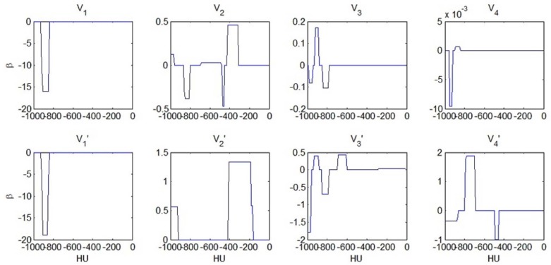
3 is generally a concave function between −950 HU and −600 HU, whereas it may become a convex function for abnormal scans. The physiological basis for the concavity in the normal population versus the convexity in some of the subjects with abnormal scans is an interesting future research problem. Figure 2 displays that the function estimate for the logistic regression model using V′4 V

′

4 implies the following model:

logit(p)≈constant−0.4×V′4(−1000,−900)+1.9×V′4(−800,−700)−V′4(−500,−450). logit

(

)

≈

constant

−

0.4

′

(

−

1000

−

900

)

1.9

′

(

−

800

−

700

)

−

′

(

−

500

−

450

)

Get Radiology Tree app to read full this article<

Acknowledgments

Get Radiology Tree app to read full this article<

Appendix

Get Radiology Tree app to read full this article<

p(d|vi,i∈S)×p(vi,i∈S)=p(vi,i∈S;d)=p(d)p(vi,i∈S|d)=p(d)∏i∈Sp(vi|d)={p(d)}−|S|+1∏i∈Sp(vi;d)={p(d)}−|S|+1∏i∈Sp(d|vi)p(vi) p

(

∈

)

(

∈

)

(

∈

;

)

(

)

(

∈

)

(

)

∏

∈

(

)

{

(

)

}

−

∏

∈

(

;

)

{

(

)

}

−

∏

∈

(

)

(

)

Get Radiology Tree app to read full this article<

p(D=1|vi,i∈S)p(D=0|vi,i∈S)={p(D=0)}|S|−1{p(D=1)}|S|−1∏i∈Sp(D=1|vi)p(D=0|vi), p

(

∈

)

(

∈

)

{

(

)

}

−

{

(

)

}

−

∏

∈

(

)

(

)

which becomes ∏i∈Sp(D=1|vi)p(D=0|vi) ∏

∈

(

)

(

) , the product of the posterior odds when the prior odds p(D=1)p(D=0)=1 p

(

)

(

)

1 .

Get Radiology Tree app to read full this article<

Appendix

Supplementary Material

Get Radiology Tree app to read full this article<

Figure S1

Get Radiology Tree app to read full this article<

Figure S2

Get Radiology Tree app to read full this article<

Figure S3

Get Radiology Tree app to read full this article<

Figure S4

Get Radiology Tree app to read full this article<

Figure S5

Get Radiology Tree app to read full this article<

References

1. Olson A.L., Swigris J.J., Lezotte D.C., et. al.: Mortality from pulmonary fibrosis increased in the United States from 1992 to 2003. Am J Respir Crit Care Med 2007; 176: pp. 277-284.
2. Fletcher C., Oldham P.: Problem of consistent radiological diagnosis in coalminers’ pneumoconiosis: an experimental study. Br J Ind Med 1949; 6: pp. 168.
3. Impivaara O., Zitting A.J., Kuusela T., et. al.: Observer variation in classifying chest radiographs for small lung opacities and pleural abnormalities in a population sample. Am J Ind Med 1998; 34: pp. 261-265.
4. Mulloy K.B., Coultas D.B., Samet J.M.: Use of chest radiographs in epidemiological investigations of pneumoconioses. Br J Ind Med 1993; 50: pp. 273-275.
5. Mikulski M.A., Hartley P.G., Sprince N.L., et. al.: Risk and significance of chest radiograph and pulmonary function abnormalities in an elderly cohort of former nuclear weapons workers. J Occup Environ Med 2011; 53: pp. 1046-1053.
6. Muir D., Bernholz C.D., Morgan W., et. al.: Classification of chest radiographs for pneumoconiosis: a comparison of two methods of reading. Br J Ind Med 1992; 49: pp. 869.
7. Musch D., Higgins I., Landis J.: Some factors influencing interobserver variation in classifying simple pneumoconiosis. Br J Ind Med 1985; 42: pp. 346-349.
8. Yerushalmy J., Garland L., Harkness J., et. al.: An evaluation of the role of serial chest roentgenograms in estimating the progress of disease in patients with pulmonary tuberculosis. Am Rev Tuberc 1951; 64: pp. 225-248.
9. International Labour Organization (ILO) : Guidelines for the use of the ILO international classification of radiographs of pneumoconioses.Occupational Safety and Health Series No. 222002.International Labour Office, ILOGeneva Rev 2000
10. National Institute of Occupational Safety and Health. (NIOSH) : Issues in classification of chest radiographs. NIOSH.2010.Centers for Disease Control and Prevention (CDC)Atlanta, GA
11. Busacker A., Newell J.D., Keefe T., et. al.: A multivariate analysis of risk factors for the air-trapping asthmatic phenotype as measured by quantitative CT analysis. Chest 2009; 135: pp. 48-56.
12. Al Jarad N., Poulakis N., Pearson M., et. al.: Assessment of asbestos-induced pleural disease by computed tomography—correlation with chest radiograph and lung function. Respir Med 1991; 85: pp. 203-208.
13. Bessis L., Callard P., Gotheil C., et. al.: High-resolution CT of parenchymal lung disease: precise correlation with histologic findings. Radiographics 1992; 12: pp. 45-58.
14. Friedman A.C., Fiel S.B., Fisher M.S., et. al.: Asbestos-related pleural disease and asbestosis: a comparison of CT and chest radiography. AJR Am J Roentgenol 1988; 150: pp. 269-275.
15. Harkin T.J., McGuinness G., Goldring R., et. al.: Differentiation of the ILO boundary chest roentgenograph (0/1 to 1/0) in asbestosis by high-resolution computed tomography scan, alveolitis, and respiratory impairment. J Occup Environ Med 1996; 38: pp. 46-52.
16. Mathieson J., Mayo J., Staples C., et. al.: Chronic diffuse infiltrative lung disease: comparison of diagnostic accuracy of CT and chest radiography. Radiology 1989; 171: pp. 111-116.
17. Ochsmann E., Carl T., Brand P., et. al.: Inter-reader variability in chest radiography and HRCT for the early detection of asbestos-related lung and pleural abnormalities in a cohort of 636 asbestos-exposed subjects. Int Arch Occup Environ Health 2010; 83: pp. 39-46.
18. Flohr T.G., Schaller S., Stierstorfer K., et. al.: Multi–detector row CT systems and image-reconstruction techniques 1. Radiology 2005; 235: pp. 756-773.
19. Kalra M.K., Maher M.M., Toth T.L., et. al.: Techniques and applications of automatic tube current modulation for CT 1. Radiology 2004; 233: pp. 649-657.
20. Hoffman E.A., Lynch D.A., Barr R.G., et. al.: Pulmonary CT and MRI phenotypes that help explain chronic pulmonary obstruction disease pathophysiology and outcomes. J Magn Reson Imaging 2015; Epub ahead of print
21. Guo J., Fuld M.K., Alford S.K., et. al.: Pulmonary Analysis Software Suite 9.0: Integrating quantitative measures of function with structural analyses. First International Workshop on Pulmonary Image Analysis2008.pp. 283-292.
22. Hu S., Hoffman E.A., Reinhardt J.M.: Automatic lung segmentation for accurate quantitation of volumetric X-ray CT images. IEEE Trans Med Imaging 2001; 20: pp. 490-498.
23. Tibshirani R., Saunders M., Rosset S., et. al.: Sparsity and smoothness via the fused lasso. J R Stat Soc Series B Stat Methodol 2005; 67: pp. 91-108.
24. MATLAB and Statistics Toolbox Release 2013b, The MathWorks, Inc., Natick, Massachusetts, United States.
25. Liu J., Ji S., Ye J.: SLEP: sparse learning with efficient projections. Arizona State University2009.
26. Gattinoni L., Caironi P., Pelosi P., et. al.: What has computed tomography taught us about the acute respiratory distress syndrome?. Am J Respir Crit Care Med 2001; 164: pp. 1701-1711.
27. Lynch D.A., Godwin J.D., Safrin S., et. al.: High-resolution computed tomography in idiopathic pulmonary fibrosis: diagnosis and prognosis. Am J Respir Crit Care Med 2005; 172: pp. 488-493.
28. Hartley P.G., Galvin J.R., Hunninghake G.W., et. al.: High-resolution CT-derived measures of lung density are valid indexes of interstitial lung disease. J Appl Physiol 1994; 76: pp. 271-277.
29. Yilmaz C., Watharkar S.S., de Leon A.D., et. al.: Quantification of regional interstitial lung disease from CT-derived fractional tissue volume: a lung tissue research consortium study. Acad Radiol 2011; 18: pp. 1014-1023.

Novel Logistic Regression Model of Chest CT Attenuation Coefficient Distributions for the Automated Detection of Abnormal (Emphysema or ILD) Versus Normal Lung

Rationale and Objectives

Materials and Methods

Results

Conclusions

Materials and Methods

Data

Logistic Regression Model

The fused-lasso estimator

Misclassification Rates

Information Pooling

Results

Discussion

Acknowledgments

Appendix

Appendix

Supplementary Material

References

Further Reading

Advances in the Treatment of Oligometastatic Disease

Assessment of Background Parenchymal Enhancement and Lesion Kinetics in Breast MRI of BRCA 1/2 Mutation Carriers Compared to Matched Controls Using Quantitative Kinetic Analysis

Automated Assessment of Left Ventricular Function and Mass Using Heart Deformation Analysis