On the Convexity of ROC Curves Estimated from Radiological Test Results

Rationale and Objectives

Although an ideal observer’s receiver operating characteristic (ROC) curve must be convex—ie, its slope must decrease monotonically—published fits to empirical data often display “hooks.” Such fits sometimes are accepted on the basis of an argument that experiments are done with real, rather than ideal, observers. However, the fact that ideal observers must produce convex curves does not imply that convex curves describe only ideal observers. This article aims to identify the practical implications of nonconvex ROC curves and the conditions that can lead to empirical or fitted ROC curves that are not convex.

Materials and Methods

This article views nonconvex ROC curves from historical, theoretical, and statistical perspectives, which we describe briefly. We then consider population ROC curves with various shapes and analyze the types of medical decisions that they imply. Finally, we describe how sampling variability and curve-fitting algorithms can produce ROC curve estimates that include hooks.

Results

We show that hooks in population ROC curves imply the use of an irrational decision strategy, even when the curve does not cross the chance line, and therefore usually are untenable in medical settings. Moreover, we sketch a simple approach to improve any nonconvex ROC curve by adding statistical variation to the decision process. Finally, we sketch how to test whether hooks present in ROC data are likely to have been caused by chance alone and how some hooked ROCs found in the literature can be easily explained as fitting artifacts or modeling issues.

Conclusion

In general, ROC curve fits that show hooks should be looked on with suspicion unless other arguments justify their presence.

The history of science is the story of cyclical interaction between theoretical models and experiments. The present article is concerned with the science of binary decision making under uncertainty and, in particular, the perspectives of receiver operating characteristic (ROC) analysis that provide a conceptual basis for nearly all applications of that science. Contemporary introductions to ROC methodology have been provided by Pepe , Zhou et al , and Wagner et al , for example.

A principal purpose of this article is to call attention to recent refinements in the understanding of ROC models in diagnostic imaging and clinical laboratory testing. These refinements have come about through more careful scrutiny of observed data, new developments in mathematical modeling and data analysis, and a recognition of potential logical inconsistencies in the common applications and interpretations of what has become the most popular ROC paradigm. Some new developments will be recapitulated here; logical difficulties are then identified and our proposed resolution of them presented. Although our view is by no means revolutionary, we believe that it goes beyond incremental refinement. In particular, we begin by shifting attention from the diagnostic performance observed in a particular experiment to the information that such experiments provide concerning potentially improved future implementations of the technologies tested, in part because it would be unethical to discard a new diagnostic test merely on the grounds that it was employed inappropriately in a particular experiment (eg, interpreted by observers who did not have adequate experience with the test) or judged to perform poorly because of an evaluation methodology artifact that should have been anticipated or corrected.

Get Radiology Tree app to read full this article<

Materials and methods

Some Historical Perspective: The National Cancer Institute Initiative of the late 1970s

Get Radiology Tree app to read full this article<

$Figure 1, Examples of receiver operating curve (ROC) curves plotted together with the chance line ( dot-dashed gray line ). Displayed here are a generic convex ROC curve ( black ), a nonconvex curve with a hook but not crossing the chance-line ( dotted line ), a nonconvex curve that crosses the chance-line ( medium dashed line ) and a curve that decreases, thus not being a properly defined ROC curve ( long-dashed line ); see text. TPF, true-positive fraction; FPF, false-positive fraction.$

Get Radiology Tree app to read full this article<

Definitions of Basic Concepts

Get Radiology Tree app to read full this article<

FPF=1−F(v|−)andTPF=1−F(v|+) F

−

(

−

)

and

−

(

)

for any v , where F is the cumulative distribution function of the random variable v over the population of interest , conditional on the actual presence or absence of the medical condition in question, indicated with “+” and “-”, respectively. Throughout, we use v to denote both latent and actual decision variables unless explicit distinction between the two seems necessary to avoid confusion.

Get Radiology Tree app to read full this article<

Results

Population ROC Curves

Get Radiology Tree app to read full this article<

Random Decisions are Associated with Straight Lines

Get Radiology Tree app to read full this article<

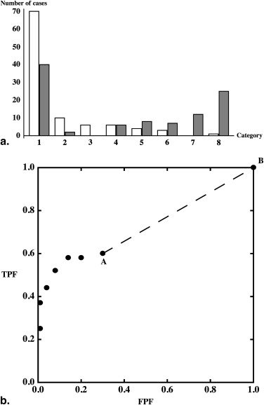
TPF=TPFA+(FPF−FPFA)(q/p). T

(

−

)

(

)

Different values of λ will produce different points on what is obviously a straight line, indicated in the plot by a dashed line segment, and we can operate at any point on this straight line between A and B by choosing an appropriate value of λ with which to compare outcomes of the random variable r . The procedure that we have described here makes no use of particular characteristics of the points A and B, so we can generalize our results in two ways. First, any discrete set of meaningful ROC points—points that represent cumulative probabilities of a decision variable —can be transformed into a well-defined and unique continuous ROC curve without using additional data: even if the decision variable is in fact discrete, we can work as if a continuous decision variable v were used to construct a continuous ROC curve through any set of ROC points. Second, if decisions are made randomly within any interval (eg, v1<v≤v2 v

≤

2 ), the resulting ROC curve will be a straight line for the curve points corresponding to that interval. If all decisions are made randomly for all cases in the selected population, then FPF A = TPF A = 0and p = q = 1, so the line is the positive diagonal of ROC space, the already introduced and well-known chance line.

$Figure 2, ( Upper panel ) Bar chart of a simulated eight-category contaminated dataset. Actually negative cases are displayed as white bars; actually positive cases are displayed as gray bars. Cases in categories with a larger index have a higher probability of being actually positive according to the hypothetical decision process we are simulating. Contamination can be observed in the category labeled “1.” ( Lower panel ) The same dataset displayed as a receiver operating characteristic plot. TPF: true-positive fraction; FPF: false-positive fraction.$

Get Radiology Tree app to read full this article<

(FPFC,TPFC)=(FPFA+λCp,TPFA+λCq), (

)

(

)

where p and q are defined as before and λ C is the value of λ that defines the coordinates of point C. From equation , it follows that the conditional cumulative distribution functions for the decision variable v , evaluated at the value v C that yields the operating point C, must satisfy the simple relationships

F(vC|+)=1−TPFA−λCqandF(vC|−)=1−FPFA−λCp, F

(

)

−

and

(

−

)

−

F(vC|+)=constant+F(vC|−)q/p F

(

)

constant

(

−

)

and the conditional density functions must satisfy

f(vC|+)/f(vC|−)=q/p. f

(

)

(

−

)

The ratio on the left side of the latter equation is the previously encountered likelihood ratio. Accordingly, all cases with test result values that correspond to thresholds on the straight-line segment have the same odds, and thus the same probability, of being actually positive , independent of the value of λ c or v C . Using v to separate actually positive from actually negative cases is equivalent to making random decisions for that interval: changing the value of v is equivalent to changing the value of λ in the random decision process described in the previous paragraph. The chance line is simply equivalent to an exclusively random decision process in v : different values of the variable v always contain the same information about the condition of interest—the prevalence.

Get Radiology Tree app to read full this article<

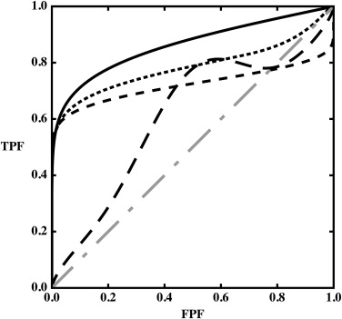
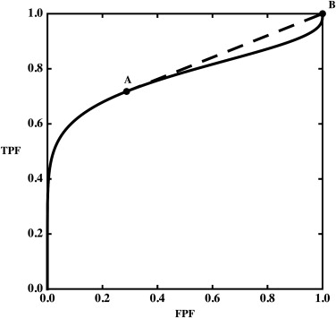
“Hooks,” Convex ROC Curves, and Straight Lines

Get Radiology Tree app to read full this article<

$Figure 3, Two operating points, A and B, are shown on a hooked receiver operating characteristic curve. The dashed straight line segment between A and B reveals a hook that drops below it. TPF, true-positive fraction; FPF, false-positive fraction.$

Get Radiology Tree app to read full this article<

ROC Curves Estimated from Samples

Get Radiology Tree app to read full this article<

Populations with Convex ROC Curves can Produce Empirical ROCs with Hooks

Get Radiology Tree app to read full this article<

How Nonconvex ROC Curve Fits Usually Happen

Get Radiology Tree app to read full this article<

Conclusions

Get Radiology Tree app to read full this article<

$Figure 4, Empirical operating points ( diamonds ) and the fitted receiver operating characteristic (ROC) curve ( solid ) for synthetic data generated from Figure 1 (d) in reference (34) , which describes the estimated performance of film mammography in screening for breast cancer in premenopausal or perimenopausal women. Both vertical and horizontal 95% confidence intervals for the operating points are shown by bars, but the horizontal bars are invisible here because of their very small size. Point H is the operating point on the ROC curve at which the tangent to the fitted ROC curve passes through (1,1) (ie, the beginning of the hook), according to the definition employed in this article. The tangent at H is shown as a dashed straight line segment. TPF: true-positive fraction; FPF: false-positive fraction.$

Get Radiology Tree app to read full this article<

Acknowledgment

Get Radiology Tree app to read full this article<

Appendix 1 An algorithm to judge whether a hook is real

Get Radiology Tree app to read full this article<

TPFB<TPFA+(FPFB−FPFA)(TPFC−TPFA)(FPFC−FPFA), T

(

−

)

(

−

)

(

−

)

given that FPFA<FPFB<FPFC F

C . Thus, point B must lie below the straight line connecting A with C. It is straightforward to generalize this to a sequence of points, all of which lie below the segment connecting two points, A and B, or to a dataset with multiple hooks.

Get Radiology Tree app to read full this article<

(lj/Ms)/(kj/Mn)<(lj−1/Ms)/(kj−1/Mn) (

)

(

)

(

−

)

(

−

)

for at least some category j, where Mn=∑Ncatj=1kj M

∑

j and Ms=∑Ncatj=1lj M

∑

j . A population ROC indistinguishable from that of the sampled data can be defined by assigning the population probabilities pj=kj/Mn p

n and qj=lj/Ms q

s to every category j, thereby causing the hypothetical population of test results to be categorical as well; thus, condition (A1.2) implies that

qj/pj<qj−1/pj−1. q

−

Notice that we have defined empirical ROC curves in terms of numbers of cases, whereas we have defined population ROC curves in terms of probability distributions.

Get Radiology Tree app to read full this article<

Appendix 2 How Hooks can Happen and a Way to Reconsider Them, with an Example from Published Data

Get Radiology Tree app to read full this article<

P(k→,l→∣∣α,β,x→)=Mn!Ms!∏5i=1pkiiqliiki!li!, P

(

→

)

∏

where α and β are the parameters that specify the population ROC curve according to a particular model; k i and l i are the numbers of actually negative and actually positive cases in category i , respectively; Mn=∑5i=1ki M

∑

i ; Ms=∑5i=1li M

∑

i ; and the vector ν→ ν

→ represents an ordered set of category boundaries that defines the conditional response probabilities associated with each category via the equations

pi=p(α,β,νi−1,νi)=P(ni−1≤ν≤νi|α,β,−) p

(

−

)

(

−

≤

−

)

and

qi=q(α,β,νi−1,νi)=P(ni−1≤ν≤νi|α,β,+), q

(

−

)

(

−

≤

)

in which ν is the latent decision variable (see Metz for details) . The “best fit” ROC curve usually is determined by maximum-likelihood estimation (MLE) because of its good statistical properties . Each such ROC curve estimate consists of the values of α , β , and ν→ ν

→ that maximize the value of an appropriate likelihood function. Usually, a modified log-likelihood function is employed for numerical and other practical reasons :

LL(k→,l→∣∣α,β,ν→)=∑5i=1kilogpi+lilogqi. L

(

→

)

∑

log

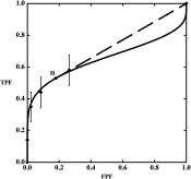
We created artificial data based on Figure 1 (d) in , which represents the ROC curve of film mammography screening for premenopausal or perimenopausal women. We chose to synthesize data on the basis of information in this publication because it reports a large clinical trial in which data were collected by experienced investigators under carefully controlled conditions. We chose the particular dataset shown in Figure 1 (d) in because it displays the most obvious hook. The original data were collected on a seven-category scale, but we simplified them to five-category data because the first three ROC operating points are essentially aligned vertically, thereby allowing the corresponding categories to be merged without affecting the maximum-likelihood estimates of the ROC curve . We measured the false-positive fraction (FPF) and true -positive fraction (TPF) values as accurately as possible from the published plot and synthesized data from similar numbers of actually positive and actually negative cases, as in . The resulting synthesized dataset consisted of test result values for 100 actually positive cases and 16,000 actually negative cases. This is a highly unbalanced dataset, as is often the case in prospective clinical trials that assess the detection of diseases with low prevalence. The empirical operating points and the corresponding ROC curve estimated by our LABROC4 algorithm for fitting the conventional binormal model (available on request from http://www-radiology.uchicago.edu/krl/ ) are shown in Figure 4 . Our fitted curve is somewhat lower and displays a slightly more obvious hook than the original because the samples are slightly different. The standard errors of our resulting parameter estimates were similar to those reported in .

Get Radiology Tree app to read full this article<

References

1. Pepe M.S.: The statistical evaluation of medical tests for classification and prediction.2004.Oxford University PressOxford; New York
2. Zhou X.-H., Obuchowski N.A., McClish D.K.: Statistical methods in diagnostic medicine.2002.Wiley-InterscienceNew York, NY
3. Wagner R.F., Metz C.E., Campbell G.: Assessment of medical imaging systems and computer aids: a tutorial review. Acad Radiol 2007; 14: pp. 723-748.
4. Swets J.A., Pickett R.M., Whitehead S.F., et. al.: Assessment of diagnostic technologies. Science 1979; 205: pp. 753-759.
5. Swets J.A., Pickett R.M.: Evaluation of diagnostic systems: methods from signal detection theory.1982.Academic PressNew York, NY
6. Dorfman D.D., Alf E.: Maximum-likelihood estimation of parameters of signal-detection theory and determination of confidence intervals—rating method data. J Math Psychol 1969; 6: pp. 487-496.
7. Metz C.E., Kronman H.B.: Statistical significance tests for binormal ROC curves. J Math Psychol 1980; 22: pp. 218-243.
8. Metz C.E., Wang P.-L., Kronman H.B.: A new approach for testing the significance of differences between ROC curves measured from correlated data.Deconinck F.Information processing in medical imaging.1984.NijhoffThe Hague, The Netherlands:pp. 432.
9. Metz C.E., Herman B.A., Roe C.A.: Statistical comparison of two ROC-curve estimates obtained from partially-paired datasets. Med Decis Making 1998; 18: pp. 110-121.
10. Henkelman R.M., Kay I., Bronskill M.J.: Receiver operator characteristic (ROC) analysis without truth. Med Decis Making 1990; 10: pp. 24-29.
11. Fryback D.G., Thornbury J.R.: The efficacy of diagnostic imaging. Med Decis Making 1991; 11: pp. 88-94.
12. International Commission on Radiation Units and Measurements: Receiver Operating Characteristic Analysis in Medical Imaging (ICRU Report 79). J ICRU 2008; 8: pp. 1-62.
13. Swets J.A.: Indices of discrimination or diagnostic accuracy: their ROCs and implied models. Psychol Bull 1986; 99: pp. 100-117.
14. Swets J.A.: Form of empirical ROCs in discrimination and diagnostic tasks: implications for theory and measurement of performance. Psychol Bull 1986; 99: pp. 181-198.
15. Hanley J.A.: Receiver operating characteristic (ROC) methodology: the state of the art. Crit Rev Diagn Imaging 1989; 29: pp. 307-335.
16. Hanley J.A.: The robustness of the “binormal” assumptions used in fitting ROC curves. Med Decis Making 1988; 8: pp. 197-203.
17. Green D.M., Swets J.A.: Signal detection theory and psychophysics.1966.WileyNew York, NY
18. Metz C.E., Pan X.: “Proper” binormal ROC curves: theory and maximum-likelihood estimation. J Math Psychol 1999; 43: pp. 1-33.
19. Dorfman D.D., Berbaum K.S., Metz C.E., et. al.: Proper receiver operating characteristic analysis: the bigamma model. Acad Radiol 1997; 4: pp. 138-149.
20. Dorfman D.D., Berbaum K.S.: A contaminated binormal model for ROC data. Part II: a formal model. Acad Radiol 2000; 7: pp. 427-437.
21. Pesce L.L., Metz C.E.: Reliable and computationally efficient maximum-likelihood estimation of “proper” binormal ROC curves. Acad Radiol 2007; 14: pp. 814-829.
22. Lloyd C.J.: Estimation of a convex ROC curve. Stat Prob Lett 2002; 59: pp. 99-111.
23. Egan J.P.: Signal detection theory and ROC analysis.1975.Academic PressNew York, NY
24. Rosen K.H.: Discrete mathematics and its applications.6th ed.2007.McGraw-Hill Higher EducationBoston, Ma
25. American College of Radiology: Breast imaging reporting and data system (BI-RADS).2003.American College of RadiologyReston, Va
26. Papoulis A.: Probability, random variables, and stochastic processes.2nd ed.1984.McGraw-HillNew York, NY
27. Anderson W.F., Reiner A.S., Matsuno R.K., et. al.: Shifting breast cancer trends in the United States. J Clin Oncol 2007; 25: pp. 3923-3929.
28. Beiden S.V., Campbell G., Meier K.L., et. al.: On the problem of ROC analysis without truth: the EM algorithm and the information matrix. Proc SPIE 2000; 3981: pp. 126-134.
29. Lang S.: Undergraduate analysis.2nd ed.1997.SpringerNew York, NY
30. Metz C.E.: Some practical issues of experimental design and data analysis in radiological ROC studies. Invest Radiol 1989; 24: pp. 234-245.
31. Birdsall TG. The theory of signal detectability: ROC curves and their character. Doctoral thesis. Ann Arbor: University of Michigan, 1966.
32. Swensson R.G., King J.L., Gur D.: A constrained formulation for the receiver operating characteristic (ROC) curve based on probability summation. Med Phys 2001; 28: pp. 1597-1609.
33. Kendall M.G., Stuart A., Ord J.K., et. al.: Kendall’s advanced theory of statistics.6th ed.1994.Edward Arnold; Halsted PressLondon, UK
34. Pisano E.D., Gatsonis C., Hendrick E., et. al.: Diagnostic performance of digital versus film mammography for breast-cancer screening. N Engl J Med 2005; 353: pp. 1773-1783.
35. Ogilvie J., Creelman C.D.: Maximum likelihood estimaton of receiver operating characteristic curve parameters. J Math Psychol 1968; 5: pp. 377-391.
36. Metz C.E.: Statistical analysis of ROC data in evaluating diagnostic performance.Herbert D.E.Myers R.H.Multiple regression analysis: applications in the health sciences.1986.American Institute of Physics: American Association of Physicists in MedicineNew York, NY:pp. 365-384.
37. Metz C.E., Herman B.A., Shen J.H.: Maximum likelihood estimation of receiver operating characteristic (ROC) curves from continuously-distributed data. Stat Med 1998; 17: pp. 1033-1053.

On the Convexity of ROC Curves Estimated from Radiological Test Results

Rationale and Objectives

Materials and Methods

Results

Conclusion

Materials and methods

Some Historical Perspective: The National Cancer Institute Initiative of the late 1970s

Definitions of Basic Concepts

Results

Population ROC Curves

Random Decisions are Associated with Straight Lines

“Hooks,” Convex ROC Curves, and Straight Lines

ROC Curves Estimated from Samples

Populations with Convex ROC Curves can Produce Empirical ROCs with Hooks

How Nonconvex ROC Curve Fits Usually Happen

Conclusions

Acknowledgment

Appendix 1

An algorithm to judge whether a hook is real

Appendix 2

How Hooks can Happen and a Way to Reconsider Them, with an Example from Published Data

References

Further Reading

CADe Prompts and Observer Performance

CT Colonography Computer-Aided Polyp Detection

Curriculum Development For Medical Education A Six-Step Approach, 2nd Edition