On the Shape of the Population ROC Curve

Rationale and Objectives

Human observers often do not produce empirical operating points near the northeast corner of the receiver operating characteristic (ROC) plot, and thus the local shape of the population ROC curve is unknown.

Materials and Methods

We call attention to occult abnormalities and propose that considerations by human observers of the prior probability of occult abnormalities can cause the shape of the local population ROC curve to be convex, a straight line, or concave near the northeast corner of the ROC plot. We further conducted a set of simulated detection-task (without-search) experiments with human observers and, mathematically, with an ideal observer and a model observer. In the experiments, we used signals, pseudo-signals that were similar to signals, and random image noise. The relative frequency of occult signals was controlled in the experiments.

Results

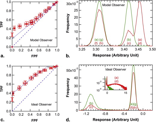
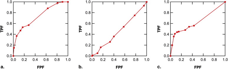
In the simulated experiments, the population ROC curve of the ideal observer was always convex, but those of the model observer and of human observers were convex, a straight-line, or concave, depending on the relative frequency of occult signals. The population ROC curve for the model observer was identical to that for the ideal observer when knowing the relative frequency of occult signals was not important for the ideal observer, and it was similar to that for human observers otherwise.

Conclusion

Observer consideration of the prior probability of occult abnormalities is important in ROC studies and could cause unexpected shapes of the local population ROC curve. Absence of empirical operating points near the northeast corner of the ROC plot may be caused by occult abnormalities.

Receiver operating characteristic (ROC) analysis is widely used for characterizing the decision-making performance in binary discrimination tasks, particularly those that involve medical imaging systems and expert human observers such as radiologists . An important goal of ROC analysis is to obtain an estimate of the population ROC curve based on empirical operating points (ie, sensitivity-specificity pairs) derived from a radiologist’s confidence ratings that a specified abnormality is present in each case of a set of images. It has long been known that empirical operating points tend to be absent near the northeast corner of the ROC plot . An example of this is the Digital Mammography Imaging Screening Trial (DMIST) . In the data shown in Figure 1 , the large space near the northeast corner of the ROC plot that is devoid of empirical operating points can be problematic for parametric ROC curve estimation, and the conventional and the proper binormal models can yield quite different ROC curve estimates.

Open full size image

Figure 1

Conventional and proper binormal model receiver operating characteristic (ROC) curve estimates for two sub-datasets from the Digital Mammography Imaging Screening Trial: (a) screen-film mammogram data of 42,745 women with 335 verified breast cancers (from Fig 1 a and table 3 of reference ); and (b) screen-film mammogram data of 15,803 premenopausal or perimenopausal women with 100 verified breast cancers (from Fig 1 d and table 2 of reference ). Maximum-likelihood area under the ROC curve (AUC) estimates (± standard error) based on the proper and conventional binormal models are also shown. FPF, false-positive fraction; TPF, true-positive fraction.

Get Radiology Tree app to read full this article<

Open full size image

Figure 2

Schematic illustration of a population receiver operating characteristic curve that has a local segment near the northeast corner of: (a) convex shape, as illustrated by the points A-X-B; (b) straight line, as illustrated by the points A-Y-B; and (c) concave shape, as illustrated by the points A-Z-B. FPF, false-positive fraction; TPF, true-positive fraction.

Get Radiology Tree app to read full this article<

Materials and methods

Conceptual Analysis

Empirical evidence and prior probability

Get Radiology Tree app to read full this article<

Occult abnormalities

Get Radiology Tree app to read full this article<

Locally straight-line ROC curve segment

Get Radiology Tree app to read full this article<

Locally convex ROC curve segment

Get Radiology Tree app to read full this article<

Locally concave ROC curve segment

Get Radiology Tree app to read full this article<

Simulation Study

Get Radiology Tree app to read full this article<

The detection task

Get Radiology Tree app to read full this article<

Three experiments

Get Radiology Tree app to read full this article<

Table 1

Composition of Simulated Images in Three Experiments

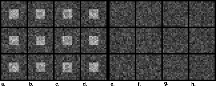
Relative Frequency (%) of Signal (S) and Pseudo-signal (PS) in Simulated Image Sets Image Column ∗ (a) (b) (c) (d) (e) (f) (g) (h) Composition H-S, N-PS N-S, H-PS L-S, H-PS H-S, L-PS N-S, N-PS L-S, N-PS N-S, L-PS L-S, L-PS 1-D profile † Experiment I 19 45 25 6 5 0 0 0 Experiment II 0 0 0 0 5 25 45 25 Experiment III 15 22.5 7.5 5 5 15 22.5 7.5

See Figure 3 for example images.

H, high magnitude; L, low magnitude; N, no (ie, magnitude = zero); PS, pseudo-signal; S, signal.

Get Radiology Tree app to read full this article<

Human observer experiment

Get Radiology Tree app to read full this article<

Ideal observer and model observer

Get Radiology Tree app to read full this article<

Data Analysis

Get Radiology Tree app to read full this article<

Results

Get Radiology Tree app to read full this article<

$Figure 5, Model observer and ideal observer results in Experiment I: (a) empirical operating points of the model observer, (b) histograms of the model observer's responses, (c) empirical operating points of the ideal observer, and (d) histograms of the ideal observer's responses. In (d) , the main plot shows a truncated version of the histograms of the ideal observer's responses, and the two inserts show the full histograms in a semi-log plot, demonstrating long tails that correspond to operating points (not shown in (c) ) with FPF ≈0 ≈0 and with TPF ≈1 ≈1 . In (a) and (c) , the dashed lines show chance performance. In (c) and (d) , the red curves correspond to signal-present images; the green curves correspond to signal-absent images. FPF, false-positive fraction; TPF, true-positive fraction.$

Get Radiology Tree app to read full this article<

$Figure 6, Model observer and ideal-observer results in Experiment II: (a) empirical operating points of the model observer, (b) histograms of the model observer's responses, (c) empirical operating points of the ideal observer, and (d) histograms of the ideal observer's responses. In (d) , the main plot shows a close-up view of the histograms of the ideal observer's responses; the insert shows the histograms in a semi-log plot, both in the same scales as in Figure 5 (d) for comparison. In (a) and (c) , the dashed lines show chance performance. In (c) and (d) , the red curves correspond to signal-present images; the green curves correspond to signal-absent images. FPF, false-positive fraction; TPF, true-positive fraction.$

Get Radiology Tree app to read full this article<

$Figure 7, Model observer and ideal observer results in Experiment III: (a) empirical operating points of the model observer, (b) histograms of the model observer's responses, (c) empirical operating points of the ideal observer, and (d) histograms of the ideal observer's responses. In (d) , the main plot shows a truncated version of the histograms of the ideal observer's responses, and the insert shows the full histograms in a semi-log plot, demonstrating long tails that correspond to operating points (not shown in c ) with FPF ≈0 ≈0 . In (a) and (c) , the dashed lines show chance performance; the dotted lines have a slope of 22.5/27.5, which is the proportion of signal-present images in “nothing-apparently-present” images ( Fig 3 image columns e–h , and Table 1 ). In (c) and (d) , the red curves correspond to signal-present images; the green curves correspond to signal-absent images. FPF, false-positive fraction; TPF, true-positive fraction.$

Get Radiology Tree app to read full this article<

$Figure 8, Typical human-observer empirical operating points in (a) Experiment I, (b) Experiment II, and (c) Experiment III. FPF, false-positive fraction; TPF, true-positive fraction.$

Get Radiology Tree app to read full this article<

Discussion

Get Radiology Tree app to read full this article<

Acknowledgments

Get Radiology Tree app to read full this article<

Appendix

Simulated Image

Get Radiology Tree app to read full this article<

s=Ms×{1,0,center7×7=49pixelseverywhereelse s

{

center

pixels

everywhere

else

f=Mf×⎧⎩⎨⎪⎪1,F,0,center7×7=49pixelsexceptforcenter3×3=9pixelscenter3×3=9pixelseverywhere else f

{

center

pixels

except

for

center

pixels

center

pixels

everywhere else

and

g˜=Mn×N(0,σ), g

(

)

where Ms M

s , Mf M

f , and Mn M

n are the magnitude of signal s s , pseudo-signal f f , and noise g˜ g

˜ , respectively, and F<1 F

1 is a fixed constant fraction of Mf M

f . Then,

x˜=⎧⎩⎨⎪⎪⎪⎪⎪⎪⎪⎪⎪⎪⎪⎪⎪⎪⎪⎪⎪⎪⎪⎪⎪⎪⎪⎪⎪⎪⎪⎪⎪⎪⎪⎪⎪⎪b+s+g˜,(signal−present)orb+s+f+g˜,(signal−present)orb+g˜,(signal−absent)orb+f+g˜,(signal−absent). x

{

(

signal

−

present

)

(

signal

−

present

)

(

signal

−

absent

)

(

signal

−

absent

)

Get Radiology Tree app to read full this article<

Ideal Observer

Get Radiology Tree app to read full this article<

L(x˜|s)=∑iL(x˜|s*i)p(s*i)∑ip(s*i), L

(

)

∑

(

)

(

)

∑

(

)

where ∑ip(s*i)=p(s) ∑

(

)

(

) is the overall prevalence of signal-present images. Similarly, denote each distinct noiseless signal-absent image by n*i n

* , and its relative frequency in an experiment by p(n*i) p

(

) ; the likelihood of an image x˜ x

˜ conditional on signal absence is

L(x˜|n)=∑iL(x˜|n*i)p(n*i)∑ip(n*i), L

(

)

∑

(

)

(

)

∑

(

)

where ∑ip(n*i)=p(n)=1−p(s) ∑

(

)

(

)

−

(

) is the overall prevalence of signal-absent images. Therefore, the likelihood ratio of an image x˜ x

˜ is

LR(x˜)≡L(x˜|s)L(x˜|n)=∑iL(x˜|s*i)p(s*i)∑iL(x˜|n*i)p(n*i)p(n)p(s). LR

(

)

≡

(

)

(

)

∑

(

)

(

)

∑

(

)

(

)

(

)

(

)

Get Radiology Tree app to read full this article<

L(x˜∣∣s*i)=∏jMn2π√σe−(xj−μsi,j)2/2σ2, L

(

)

∏

−

(

−

)

where the index j=1,2,…,361 j

…

361 denotes each pixel in the image x˜ x

˜ , μsi,j μ

j is the corresponding pixel in the noiseless signal-present image s*i s

* , and σ2 σ

2 is the variance of the Gaussian noise. Similarly, for a single distinct noiseless signal-absent image n*i n

* ,

L(x˜∣∣n*i)=∏jMn2π√σe−(xj−μni,j)2/2σ2, L

(

)

∏

−

(

−

)

where μni,j μ

j is a single pixel in the noiseless signal-absent image n*i n

* . Thus,

LR(x˜)=p(n)p(s)∑ip(s*i)∏je−(xj−μsi,j)2/2σ2∑ip(n*i)∏je−(xj−μni,j)2/2σ2 LR

(

)

(

)

(

)

∑

(

)

∏

−

(

−

)

∑

(

)

∏

−

(

−

)

can be calculated for each image x˜ x

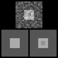
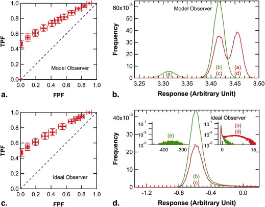
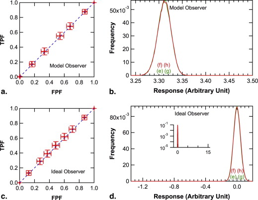
˜ , given the definitions of the signals, pseudo-signals, and their relative frequency in an experiment ( Table 1 ). lnLR(x˜) ln

(

) is plotted as the abscissa in Figures 5 d, 6 d, and 7 d separately for signal-present and signal-absent images.

Get Radiology Tree app to read full this article<

L(x˜|s*i)L(x˜|n*i)=∏je−{(xj–μsj)2−(xj–μnj)2}/2σ2=∏je{2(μsj−μnj)xj−(μ2sj–μ2nj)}/2σ2 L

(

)

(

)

∏

−

{

(

–

)

−

(

–

)

}

∏

{

(

−

)

−

(

–

)

}

ln LR(s*i,n*i)=lnL(x˜|s*i)L(x˜|n*i)=1σ2∑j(μsj−μnj)xj−12σ2∑j(μ2sj–μ2nj). ln LR

(

)

(

)

(

)

∑

(

−

)

−

∑

(

–

)

Dropping the constant term and the constant factor of the first term,

ln LR(s*i,n*i)∝∑j(μsj−μnj)xj. ln LR

(

)

∝

∑

(

−

)

Equation A12 describes an optimal filter that the ideal observer would use in an experiment that consisted of only a single distinct signal-present image and a single distinct signal-absent image before noise was added.

Get Radiology Tree app to read full this article<

Model Observer

Get Radiology Tree app to read full this article<

as−f≡cs−f(s−f),Ms=Mf a

−

≡

−

(

−

)

where cs−f c

−

f is a constant such that ∑jas−fj=1 ∑

−

1 . This filter is non-zero only in the center 3×3=9 3

9 pixels. The response of this filter to image x˜ x

˜ , Rs−f(x˜)=aTs−fx˜ R

−

(

)

−

˜ , can be calculated for each of the eight distinct noiseless images listed in Table 1 . The rank of these images in the response Rs−f(x˜) R

−

(

) from high to low is: image columns d, a, c, b, h, f, g, e ( Fig 3 ). The ideal observer response to these images can be calculated from Equation A10 . Setting all relative frequency p(⋅) p

(

⋅

) to unity, the images are ranked by the ideal observer in exactly the same order (from high response to low response: image columns d, a, c, b, h, f, g, e; Fig 3 ) under our experimental conditions (Ms1=800,Ms2=2,Mf1=800,Mf2=2,F=0.7,Mn=200,andσ=1) (

800

0.7

200

and

) . Therefore, we refer to this model observer as “perceptually optimal, or nearly optimal,” but “cognitively suboptimal.” lnRs−f(x˜) ln

−

(

) is plotted as the abscissa in Figures 5 b, 6 b, and 7 b separately for signal-present and signal-absent images.

Get Radiology Tree app to read full this article<

References

1. Metz C.E.: Basic principles of ROC analysis. Semin Nucl Med 1978; 8: pp. 283-298.
2. Wagner R.F., Metz C.E., Campbell G.: Assessment of medical imaging systems and computer aids: a tutorial review. Acad Radiol 2007; 14: pp. 723-748.
3. Pepe M.S.: The statistical evaluation of medical tests for classification and prediction.2004.Oxford University PressNew York
4. Dorfman D.D., Berbaum K.S., Brandser E.A.: A contaminated binormal model for ROC data: Part I. Some interesting examples of binormal degeneracy. Acad Radiol 2000; 7: pp. 420-426.
5. Pisano E.D., Gatsonis C., Hendrick E., et. al.: Diagnostic performance of digital versus film mammography for breast-cancer screening. N Engl J Med 2005; 353: pp. 1773-1783.
6. Metz C.E., Herman B.A., Shen J.H.: Maximum likelihood estimation of receiver operating characteristic (ROC) curves from continuously-distributed data. Stat Med 1998; 17: pp. 1033-1053.
7. Metz C.E., Pan X.: “Proper” binormal ROC curves: theory and maximum-likelihood estimation. J Math Psychol 1999; 43: pp. 1-33.
8. Pesce L.L., Metz C.E., Berbaum K.S.: On the convexity of ROC curves estimated from radiological test results. Acad Radiol 2010; 17: pp. 960-968.e4.
9. Gur D., Rockette H.E., Armfield D.R., et. al.: Prevalence effect in a laboratory environment. Radiology 2003; 228: pp. 10-14.
10. Jiang Y., Miglioretti D.L., Metz C.E., et. al.: Breast cancer detection rate: designing imaging trials to demonstrate improvements. Radiology 2007; 243: pp. 360-367.
11. Donovan T., Manning D.J.: The radiology task: Bayesian theory and perception. Br J Radiol 2007; 80: pp. 389-391.
12. Eckstein M.P., Abbey C.K., Pham B.T., et. al.: Perceptual learning through optimization of attentional weighting: human versus optimal Bayesian learner. J Vision 2004; 4: pp. 1006-1019.
13. Dorfman D.D., Berbaum K.S.: A contaminated binormal model for ROC data: Part II. A formal model. Acad Radiol 2000; 7: pp. 427-437.

On the Shape of the Population ROC Curve

Rationale and Objectives

Materials and Methods

Results

Conclusion

Materials and methods

Conceptual Analysis

Empirical evidence and prior probability

Occult abnormalities

Locally straight-line ROC curve segment

Locally convex ROC curve segment

Locally concave ROC curve segment

Simulation Study

The detection task

Three experiments

Human observer experiment

Ideal observer and model observer

Data Analysis

Results

Discussion

Acknowledgments

Appendix

Simulated Image

Ideal Observer

Model Observer

References

Further Reading

A Brief History of Free-Response Receiver Operating Characteristic Paradigm Data Analysis

An Additive Selection of Markers to Improve Diagnostic Accuracy Based on a Discriminatory Measure

An Examination of Data Confidentiality and Disclosure Issues Related to Publication of Empirical ROC Curves