Optimal Thresholds by Maximizing or Minimizing Various Metrics via ROC-Type Analysis

Rationale and Objectives

Based on imaging features, the optimal thresholds are typically determined as cutoff points to dichotomize the corresponding measurement scales.

Materials and Methods

Five metrics (ie, the Youden index, Euclidian distance, percent of correct diagnosis, kappa statistic, and mutual information) are individually maximized or minimized to derive the corresponding optimal threshold. These optimal thresholds are estimated under the parametric binormal assumption. Monte Carlo simulation studies are conducted to compare the performances of these different methods. A published radiological example on the choice of treatment outcomes following ureteral stones is used to illustrate and compare the estimated thresholds both empirically and parametrically.

Results

The optimal threshold can be a “moving target” because it would depend on modeling assumptions, metrics, and variability in the data. Even with large samples, disease prevalence has an impact on the robustness of the metrics.

Conclusions

It is recommended that researchers compare different optimal cutoff points using several metrics and select one that is most clinically relevant. The ultimate goal is to maximize diagnostic performances that are clinically meaningful to achieve improved global health.

The optimal threshold, which is also known as the operating point or cutoff point, is of importance in developing guidelines for clinical decision-making. It can be useful in practice to optimally dichotomize the measurements from an imaging feature or marker . The reason for maximizing particular metrics is that a practical and useful threshold can be critical in terms of developing medical products and therapeutics . An imaging feature can be used as a diagnostic tool for identifying patients with a disease or abnormal condition for determining the stage a disease has reached and for the prediction and monitoring of a clinical response to an intervention. Besides diagnostic imaging, optimal threshold may be useful when analyzing biomarkers .

In this article dedicated as a special tribute to Professor Charles E. Metz of the University of Chicago, we aim to extend the literature on receiver operating characteristic (ROC) analysis using optimal metrics derived from the sensitivity, specificity, agreement, distance, and information to estimate task-dependent decision criteria . We will demonstrate and investigate the thresholds that optimize Youden’s index (YI) and Euclidian distance (ED) in ROC space as well as percent correct diagnosis (PCdx), kappa ( κ ), and mutual information (MI).

Get Radiology Tree app to read full this article<

Materials and methods

Get Radiology Tree app to read full this article<

ROC Analysis

Get Radiology Tree app to read full this article<

Table 1

A Two-by-Two Table of Joint Probabilities of the Reference Standard Versus Binary Diagnosis at Each Threshold ( γ ), with Disease Prevalence π = n/N Where N = m + n

Binary Dx Based on Biomarker Measurement_RS_ Probability 0 (Healthy) 1 (Diseased) ≤ γ__p__00=_ (1 _-π_ )Sp( _γ_ )_p__01= π [1-Se(γ)]p__0●=_ (1- _π)_ Sp( _γ_ ) + _π_ [1-Se( _γ_ )] >γ_p__10= (1 -π ) [1-Sp (γ) ]p__11 = π Se( γ )p__1●=_ (1- _π)_ [1-Sp _(γ)_ ] _+ π_ Se( _γ_ ) Probability_p●0= p__00+ p__10=_ 1- _π__p●1= p__01+ p__11= π__p●0+p●1= p__0●+ p__1●__= 1

Dx, diagnosis; RS, reference standard; Sp, sensitivity; Se, specificity.

Get Radiology Tree app to read full this article<

Optimal Thresholds

Get Radiology Tree app to read full this article<

An Imaging Example

Get Radiology Tree app to read full this article<

Monte Carlo Simulations

Get Radiology Tree app to read full this article<

Results

An Imaging Example

Get Radiology Tree app to read full this article<

Table 2

Descriptive Statistics of the Ureteral Stone Sizes Measured in Millimeters Stratified by Spontaneous Passage Versus Surgical Intervention

Reference Standard Sample Size Mean SD Min Q 1 Median Q 3 Max Spontaneous passage_m_ = 71 4.18 2.10 1 3 4 5 10 Surgical intervention_n_ = 29 7.10 2.88 3 5 6 9 16

Max, maximum; min, minimum; Q 1 , 25th percentile; Q 3 , 75th percentile; SD, standard deviation.

Get Radiology Tree app to read full this article<

$Figure 1, Nonparametric and binormal receiver operating characteristic curves of ureteral stone sizes. On the x axis is the false-positive fraction (FPF) = 1-specificity (Sp) and on the y-axis is the true-positive fraction (TPF) = sensitivity (Se). Nonparametrically, the estimated specificity = 57/71 = 0.80 and sensitivity = 20/29 = 0.69, corresponding to the stone size of 5 mm as the optimal cutoff value.$

Get Radiology Tree app to read full this article<

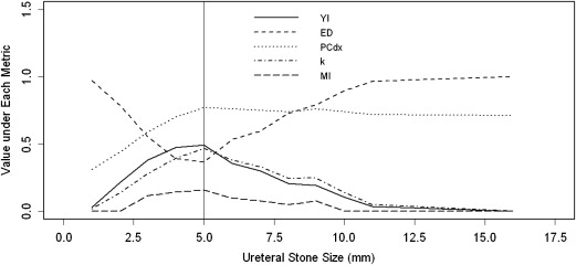
Table 3

Nonparametric Empirical Optimal Thresholds (with 95% Bootstrap Confidence Intervals) for Ureteral Stone Sizes (mm)

Optimization Metric Optimal Threshold (95% CI), mm Max (YI) 5 (3–5) Min (ED) 5 (4–5) Max (PCdx) 5 (4–6) Max ( κ ) 5 (4–6) Max (MI) 5 (3–6)

ED, Euclidian distance; κ , kappa statistic; MI, mutual information; min, minimum; max, maximum; PCdx, percent of correct diagnosis; YI = Youden index.

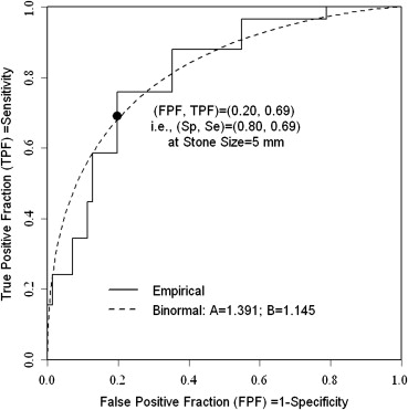
All five metrics yielded an identical optimal threshold at 5 mm. Nonparametrically, the estimated sensitivity = 0.80 and specificity = 0.69 corresponds to this cutoff value.

Get Radiology Tree app to read full this article<

Monte Carlo Simulations

Get Radiology Tree app to read full this article<

Table 4

Optimal Thresholds (with 95% Bootstrap Confidence Intervals) for Simulated Hypothetical Data Using the Equal Variance Assumption with N (0,1) and N (1,1), ie, ( α , β ) = (1, 1) Under Various Sample Sizes

Optimization Metric ( m , n ) = (200, 200) ( m , n ) = (50, 200) ( m , n ) = (200, 50) NP P NP P NP P Max (YI) 0.49 (0.04, 0.95) 0.51 (0.33, 0.67) 0.52 (−0.08, 1.11) 0.51 (0.25, 0.74) 0.47 (−0.14, 1.06) 0.52 (0.20, 0.81) Min (ED) 0.49 (0.26, 0.74) 0.50 (0.39, 0.62) 0.53 (0.20, 0.87) 0.50 (0.34, 0.67) 0.46 (0.12, 0.77) 0.51 (0.32, 0.71) Max (PCDx) 0.49 (0.04, 0.95) 0.51 (0.33, 0.67) −0.86 (−1.94, −0.26) −0.87 (−1.80, −0.36) 1.82 (1.24, 2.75) 1.89 (1.66, 2.37) Max ( κ ) 0.50 (0.04, 0.95) 0.51 (0.33, 0.67) 1.04 (0.46, 1.63) 1.03 (0.71, 1.27) −0.06 (−0.67, 0.54) −0.01 (−0.27, 0.27) Max (MI) 0.50 (−0.30, 1.31) 0.51 (0.16, 0.85) 0.70 (−0.31, 1.76) 0.67 (0.13, 1.19) 0.29 (−0.78, 1.33) 0.36 (−0.18, 0.90)

ED, Euclidian distance; κ , kappa statistic; max, maximum; MI, mutual information; min, minimum; NP, nonparametric; P, parametric; PCdx, percent of correct diagnosis; YI, Youden index.

The underlying area under the curve is 0.76.

Table 5

Optimal Thresholds (with 95% Bootstrap Confidence Intervals) for Simulated Hypothetical Data Using the Unequal Variance Assumption with N (0,1) and N (1,1/2 2 ), ie, ( α , β ) = (2, 2) Under Various Sample Sizes

Optimization Metric ( m , n ) = (200, 200) ( m , n ) = (50, 200) ( m , n ) = (200, 50) NP P NP P NP P Max (YI) 0.39 (0.16, 0.62) 0.38 (0.24, 0.54) 0.37 (0.05, 0.67) 0.39 (0.11, 0.69) 0.41 (0.10, 0.72) 0.39 (0.20, 0.57) Min (ED) 0.55 (0.40, 0.71) 0.55 (0.43, 0.68) 0.53 (0.29, 0.74) 0.56 (0.33, 0.81) 0.57 (0.37, 0.78) 0.56 (0.40, 0.72) Max (PCDx) 0.39 (0.16, 0.62) 0.38 (0.24, 0.54) −0.01 (−0.34, 0.25) −0.01 (−0.32, 0.29) 1.92 (0.81, 3.48) 1.42 (0.98, 2.87) Max ( κ ) 0.39 (0.16, 0.62) 0.38 (0.24, 0.54) 0.11 (−0.19, 0.38) 0.12 (−0.13, 0.39) 0.65 (0.32, 1.01) 0.64 (0.42, 0.85) Max (MI) 0.17 (−0.11, 0.47) 0.16 (−0.01, 0.34) 0.04 (−0.29, 0.43) 0.04 (−0.26, 0.36) 0.30 (−0.02, 0.70) 0.25 (0.02, 0.48)

ED, Euclidian distance; κ , kappa statistic; max, maximum; MI, mutual information; min, minimum; NP, nonparametric; P, parametric; PCdx, percent of correct diagnosis; YI, Youden index.

The underlying area under the curve is 0.81.

Table 6

Optimal Thresholds (with 95% Bootstrap Confidence Intervals) for Simulated Hypothetical Data Using the Unequal Variance Assumption with N (0,1) and N (1,3 2 ), ie, ( α , β ) = (1/3,1/3), Under Various Sample Sizes

Optimization Metric ( m , n ) = (200, 200) ( m , n ) = (50, 200) ( m , n ) = (200, 50) NP P NP P NP P Max (YI) 1.44 (0.98, 1.96) 1.49 (1.40, 1.58) 1.37 (0.68, 2.09) 1.50 (1.35, 1.64) 1.46 (0.80, 2.20) 1.50 (1.33, 1.63) Min (ED) 0.78 (0.44, 1.15) 0.79 (0.71, 0.87) 0.73 (0.22, 1.21) 0.79 (0.67, 0.92) 0.81 (0.32, 1.44) 0.79 (0.65, 0.93) Max (PCDx) 1.44 (0.98, 1.96) 1.49 (1.40, 1.58) −7.06 (−9.91, −5.27) −3.50 (−4.33, 0.03) 2.19 (1.61, 2.90) 2.27 (2.17, 2.36) Max ( κ ) 1.43 (0.97, 1.96) 1.49 (1.40, 1.58) 1.11 (0.37, 1.84) 1.23 (1.05, 1.39) 1.88 (1.28, 2.53) 1.91 (1.76, 2.04) Max (MI) 2.01 (1.44, 2.54) 2.12 (2.01, 2.22) 1.64 (0.98, 2.28) 1.99 (1.84, 2.14) 2.12 (1.27, 2.72) 2.32 (2.12, 2.47)

ED, Euclidian distance; κ , kappa statistic; max, maximum; MI, mutual information; min, minimum; NP, nonparametric; P, parametric; PCdx, percent of correct diagnosis; YI, Youden index.

The underlying area under the curve is 0.62.

Get Radiology Tree app to read full this article<

Discussion

Get Radiology Tree app to read full this article<

Acknowledgment

Get Radiology Tree app to read full this article<

Appendix 1 Notations and Assumptions

Get Radiology Tree app to read full this article<

Xi∼i.i.d.F(∙),∀i=1,…,m. X

∼

(

•

)

∀

…

Get Radiology Tree app to read full this article<

Yj∼i.i.d.G(∙),∀j=1,…,n. Y

∼

(

•

)

∀

…

The sample size fractions are given by

1−π=m/NforRS=0andπ=n/NforRS=1,withN=m+n, 1

−

for

and

for

,with

where π is often called the disease prevalence.

Get Radiology Tree app to read full this article<

α=(ν−μ)/τandβ=σ/τ. α

(

−

)

and

Get Radiology Tree app to read full this article<

ANP=WNP/(mn). A

(

)

Get Radiology Tree app to read full this article<

ABN=Φ(α/[(1+β2)1/2]). A

(

[

(

)

1/2

]

)

Get Radiology Tree app to read full this article<

Appendix 2 Optimal Thresholds Using Different Metrics

Get Radiology Tree app to read full this article<

γopt,YI=argmaxγ[YI(γ)],=argmaxγ[Se(γ)+Sp(γ)−1]. γ

argmax

[

(

)

]

argmax

[

(

)

(

)

−

]

A generalized YI is defined as:

GYI=Se(γ)+RSp(γ)−G, G

(

)

(

)

−

where G is a constant with respect to the threshold γ , and R = [(1- π )/ π ], a function of the disease prevalence π .

Get Radiology Tree app to read full this article<

γopt,ED=argminγ{[1−Sp(γ)−0]2+[Se(γ)−1]2}1/2,=argminγ{[Sp(γ)−1]2+[Se(γ)−1]2}1/2. γ

argmin

{

[

−

(

)

−

]

[

(

)

−

]

}

argmin

{

[

(

)

−

]

[

(

)

−

]

}

Get Radiology Tree app to read full this article<

γopt,κ=argmaxγ(p00+p11)=argmaxγ[(1−π)Sp(γ)+πSe(γ)]. γ

argmax

(

)

argmax

[

(

−

)

(

)

(

)

]

Get Radiology Tree app to read full this article<

γopt,κ=argmaxγ[2(p00p11−p10p01)/(p0∙p∙1+p∙0p1∙)]. γ

argmax

[

(

−

)

(

•

)

]

Get Radiology Tree app to read full this article<

γopt,MI=argmax[p0∙log2(p0∙)+p1∙log2(p1∙)+p∙0log2(p∙0)+p∙1log2(p∙1)−p00log2(p00)−p01log2(p01)−p10log2(p10)−p11log2(p11)], γ

arg

max

[

•

log

(

•

)

•

log

(

•

)

•

log

(

•

)

•

log

(

•

)

−

log

(

)

−

log

(

)

−

log

(

)

−

log

(

)

]

where log 2 represents log base 2.

Get Radiology Tree app to read full this article<

Appendix 3 Output Using JLABROC4

Get Radiology Tree app to read full this article<

Operating Points Corresponding to the Input Data

Get Radiology Tree app to read full this article<

Final Estimates of Binormal ROC Parameters A and B

Get Radiology Tree app to read full this article<

Area Under the ROC Curve

Get Radiology Tree app to read full this article<

References

1. Liu A., Schisterman E.F., Zhu Y.: On linear combinations of biomarkers to improve diagnostic accuracy. Stat Med 2005; 24: pp. 37-47.
2. Perkins N.J., Schisterman E.F., Vexler A.: Receiver operating characteristic curve inference from a sample with a limit of detection. Am J Epidemiol 2007; 165: pp. 325-333.
3. Perkins N.J., Schisterman E.F., Vexler A.: Generalized ROC curve inference for a biomarker subject to a limit of detection and measurement error. Stat Med 2009; 28: pp. 1841-1860.
4. Woodcock J.: Assessing the clinical utility of diagnostics used in drug therapy. Clin Pharmacol Ther 2010; 88: pp. 765-773.
5. Wagner J.A., Wright E.C., Ennis M.M., et. al.: Utility of adiponectin as a biomarker predictive of glycemic efficacy is demonstrated by collaborative pooling of data from clinical trials conducted by multiple sponsors. Clin Pharmacol Ther 2009; 86: pp. 619-625.
6. Biomarkers Definitions Working Group: Biomarkers and surrogate endpoints preferred definitions and conceptual framework. Clin Pharmacol Ther 2001; 69: pp. 89-95.
7. Lesko L.J., Atkinson A.J.: Use of biomarkers and surrogate endpoints in drug development and regulatory decision making: criteria, validation, strategies. Annu Rev Pharmacol Toxicol 2001; 41: pp. 347-366.
8. Metz C.E.: Basic principles of ROC analysis. Semin Nucl Med 1978; 8: pp. 283-298.
9. Youden W.J.: Index for rating diagnostic tests. Cancer 1950; 3: pp. 32-35.
10. Fluss R., Faraggi D., Reiser B.: Estimation of the Youden Index and its associated cutoff point. Biomed J 2005; 47: pp. 458-472.
11. Perkins N.J., Schisterman E.F.: The inconsistency of “optimal” cutpoints obtained using two criteria based on the receiver operating characteristic curve. Am J Epidemiol 2006; 163: pp. 670-675.
12. Schisterman E.F., Faraggi D., Reiser B., et. al.: Youden Index and the optimal threshold for markers with mass at zero. Stat Med 2008; 27: pp. 297-315.
13. Nakas C.T., Alonzo T.A., Yiannoutsos C.T.: Accuracy and cut-off point selection in three-class classification problems using a generalization of the Youden index. Stat Med 2010; 29: pp. 2946-2955.
14. Gönen M.: Analyzing receiver operating characteristic curves with SAS ® .2007.SAS Institute IncCary, NC
15. Zou K.H., Wells W.M., Kikinis R., et. al.: Three validation metrics for automated probabilistic image segmentation of brain tumours. Stat Med 2004; 23: pp. 1259-1282.
16. Davila M., Christenson L.J., Sontheimer R.D.: Epidemiology and outcomes of dermatology in-patient consultations in a Midwestern U.S. university hospital. Dermatol Online J 2010; 16: pp. 12.
17. Fielding J.R., Silverman S.G., Samuel S., et. al.: Unenhanced helical CT of ureteral stones: a replacement for excretory urography in planning treatment. AJR Am J Roentgenol 1998; 171: pp. 1051-1053.
18. Zou K.H., Tempany C.M., Fielding J.R., et. al.: Original smooth receiver operating characteristic curve estimation from continuous data: statistical methods for analyzing the predictive value of spiral CT of ureteral stones. Acad Radiol 1998; 5: pp. 680-687.
19. O’Malley A.J., Zou K.H., Fielding J.R., et. al.: Bayesian regression methodology for estimating a receiver operating characteristic curve with two radiologic applications: prostate biopsy and spiral CT of ureteral stones. Acad Radiol 2001; 8: pp. 713-725.
20. McClish D.K.: Evaluation of the accuracy of medical tests in a region around the optimal point. Acad Radiol 2012; 19: pp. 1484-1490.
21. Eng J.: Teaching receiver operating characteristic analysis: an interactive laboratory exercise. Acad Radiol 2012; 19: pp. 1452-1456.
22. Dorfman D.D., Alf E.: Maximum-likelihood estimation of parameters of signal-detection theory and determination of confidence intervals - rating-method data. J Math Psychol 1969; 6: pp. 487-496.
23. Metz C.E., Herman B.A., Shen J.H.: Maximum likelihood estimation of receiver operating characteristic (ROC) curves from continuously-distributed data. Stat Med 1998; 17: pp. 1033-1053.
24. Pesce L.L., Horsch K., Drukker K., et. al.: Semiparametric estimation of the relationship between ROC operating points and the test-result scale: application to the proper binormal model. Acad Radiol 2011; 18: pp. 1537-1548.
25. Alemayehu D., Zou K.H.: Applications of ROC analysis in medical research: recent developments and future directions. Acad Radiol 2012; 19: pp. 1457-1464.
26. Metz C.E.: Some practical issues of experimental design and data analysis in radiological ROC studies. Invest Radiol 1989; 24: pp. 234-245.
27. Eng J. ROC analysis: Web-based calculator for ROC curves. Available at: http://www.jrocfit.org . Accessed December 12, 2012.
28. Box G.E.P., Cox D.R.: An analysis of transformations. JRSSB 1964; 26: pp. 211-252.
29. Zou K.H., O’Malley A.J.: A Bayesian hierarchical non-linear regression model inreceiver operating characteristic analysis of clustered continuous diagnostic data. Biomed J 2005; 47: pp. 417-427.
30. O’Malley A.J., Zou K.H.: Bayesian multivariate hierarchical transformation models for ROC analysis. Stat Med 2006; 25: pp. 459-479.
31. Zou K.H., Carlsson M.O., Yu C.R.: Comparison of adjustment methods for stratified two-sample tests in the context of ROC analysis. Biomed J 2012; 54: pp. 249-263.
32. Zou K.H., Warfield S.K., Fielding J.R., et. al.: Statistical validation based on parametric receiver operating characteristic analysis of continuous classification data. Acad Radiol 2003; 10: pp. 1359-1368.
33. Hanley J.A.: Receiver operating characteristic (ROC) analysis: the state of the art. Crit Revi Diagnostic Imaging 1989; 29: pp. 307-335.
34. Hanley J.A., McNeil B.J.: The meaning and use of the area under a receiver operating characteristic (ROC) curve. Radiology 1982; 143: pp. 29-36.
35. Wieand S., Gail M.H., James B.R., et. al.: A family of nonparametric statistics for comparing diagnostic makers with paired or unpaired data. Biometrika 1989; 76: pp. 585-592.
36. Zou K.H., Liu A., Bandos A.I., et. al.: Statistical evaluation of diagnostic performance: topics in ROC analysis.2011.Chapman & Hall/CRC PressBoca Raton, FL
37. Efron B., Tibshirani R.J.: Introduction to the bootstrap.1994.Chapman & Hall/CRC PressBoca Raton, FL
38. R Development Core Team: R: a language and environment for statistical computing.2008.R Foundation for Statistical ComputingVienna, Austria Available at: http://www.R-project.org Accessed December 12, 2012
39. Robert C.P., Casella G.: Monte Carlo statistical methods.2010.Springer VerlagNew York, NY
40. Zhou X.H., Obuchowski N.A., McClish D.K.: Statistical methods in diagnostic medicine.2002.Wiley & Sons IncNew York, NY
41. Pepe M.S.: The statistical evaluation of medical tests for classification and prediction.2003.Oxford University PressOxford, UK
42. Suss R.: Sensitivity and specificity: alien edition: a light-hearted look at statistics. Can Fam Physicians 2007; 53: pp. 1743-1744.

Optimal Thresholds by Maximizing or Minimizing Various Metrics via ROC-Type Analysis

Rationale and Objectives

Materials and Methods

Results

Conclusions

Materials and methods

ROC Analysis

Optimal Thresholds

An Imaging Example

Monte Carlo Simulations

Results

An Imaging Example

Monte Carlo Simulations

Discussion

Acknowledgment

Appendix 1

Notations and Assumptions

Appendix 2

Optimal Thresholds Using Different Metrics

Appendix 3

Output Using JLABROC4

Operating Points Corresponding to the Input Data

Final Estimates of Binormal ROC Parameters A and B

Area Under the ROC Curve

References

Further Reading

A Brief History of Free-Response Receiver Operating Characteristic Paradigm Data Analysis

An Additive Selection of Markers to Improve Diagnostic Accuracy Based on a Discriminatory Measure

An Examination of Data Confidentiality and Disclosure Issues Related to Publication of Empirical ROC Curves