Performance of Breast Ultrasound Computer-aided Diagnosis

Rationale and Objectives

The automated classification of sonographic breast lesions is generally accomplished by extracting and quantifying various features from the lesions. The selection of images to be analyzed, however, is usually left to the radiologist. Here we present an analysis of the effect that image selection can have on the performance of a breast ultrasound computer-aided diagnosis system.

Materials and Methods

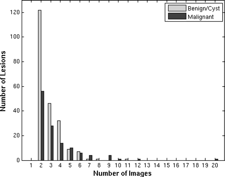
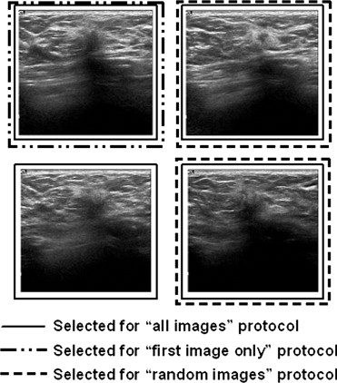
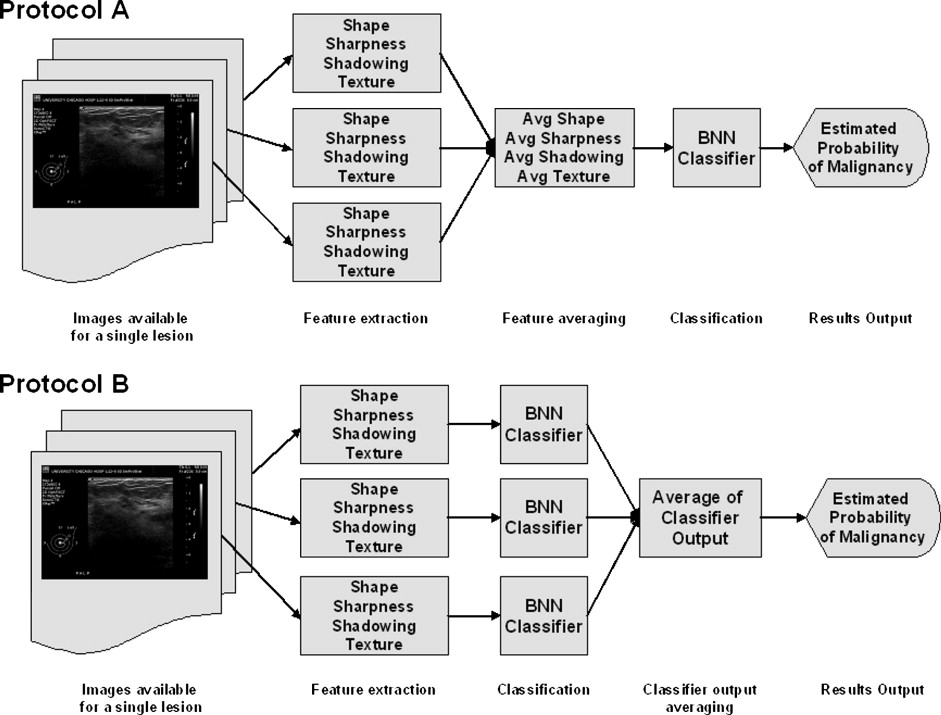
A database of 344 different sonographic lesions was analyzed for this study (219 cysts/benign processes, 125 malignant lesions). The database was collected in an institutional review board–approved, Health Insurance Portability and Accountability Act–compliant manner. Three different image selection protocols were used in the automated classification of each lesion: all images, first image only, and randomly selected images. After image selection, two different protocols were used to classify the lesions: (a) the average feature values were input to the classifier or (b) the classifier outputs were averaged together. Both protocols generated an estimated probability of malignancy. Round-robin analysis was performed using a Bayesian neural network-based classifier. Receiver-operating characteristic analysis was used to evaluate the performance of each protocol. Significance testing of the performance differences was performed via 95% confidence intervals and noninferiority tests.

Results

The differences in the area under the receiver-operating characteristic curves were never more than 0.02 for the primary protocols. Noninferiority was demonstrated between these protocols with respect to standard input techniques (all images selected and feature averaging).

Conclusion

We have proved that our automated lesion classification scheme is robust and can perform well when subjected to variations in user input.

Breast cancer continues to be the most common form of cancer and the second most common cause of death from cancer among women in the United States ( ). Although routine mammography is currently the only screening method recommended for the general public ( ), there is still considerable research being done to augment the breast cancer detection and diagnosis process. The utility of ultrasound, for example, to evaluate and diagnose lesions and abnormalities within the breast has increased dramatically over the past decade ( ). Previous studies have shown breast ultrasound to have an accuracy of 96%–100% in the diagnosis of cysts ( ) and its use in differentiating between different types of solid lesions (i.e., benign vs. malignant) is becoming more prevalent ( ). This increased interest in ultrasound as a diagnostic tool for breast cancer has led to, among other things, rapid developments in the application of computer-aided diagnosis (CADx) to breast sonography ( ).

The automated classification of sonographic breast lesions is generally accomplished by extracting and quantifying various features from the lesions. Features such as margin shape, margin sharpness, lesion texture, and posterior acoustic behavior have been shown to be particularly useful in computerized classification schemes ( ) and CADx systems based on these features have been shown to perform the benign versus malignant classification task well ( ). However, such systems are still subject to several different kinds of user-induced variability. The choice of images to be analyzed, for example, is generally left to the user of the system. As a result, the manner in which a particular lesion is input into the system may vary between different users (i.e., radiologists). This variability may have the potential to impact the output, and thus the performance, of the classifier. Here we present an analysis of the effect that image selection can have on the performance of a sonographic breast lesion CADx system.

Materials and Methods

Image Database

Get Radiology Tree app to read full this article<

Table 1

Composition of the Sonographic Database

Pathology Biopsied? No. of Patients No. of Images No. of Physical Lesions Cyst Yes 48 189 62 Cyst No 36 120 54 Benign solid/tumor Yes 63 208 68 Benign solid/tumor No 15 48 18 Benign fibrocystic Yes 15 58 17 Malignant Yes 104 444 125 Totals 281 1067 344

Get Radiology Tree app to read full this article<

Image Selection Protocols

Get Radiology Tree app to read full this article<

Lesion Classification Protocols

Get Radiology Tree app to read full this article<

Performance Assessment and Statistical Analysis

Get Radiology Tree app to read full this article<

Results

Get Radiology Tree app to read full this article<

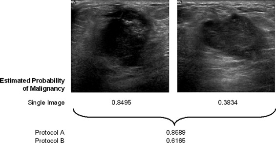
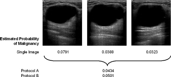
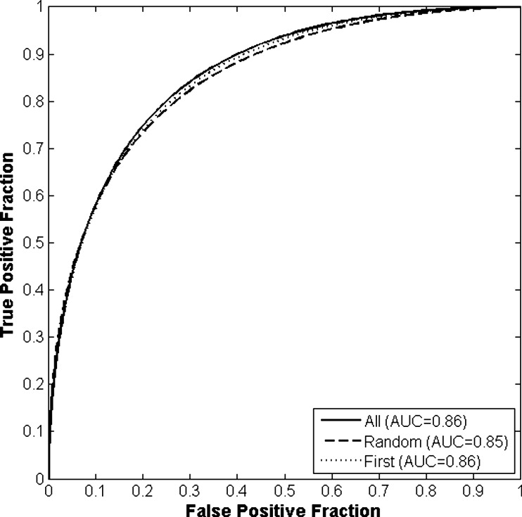
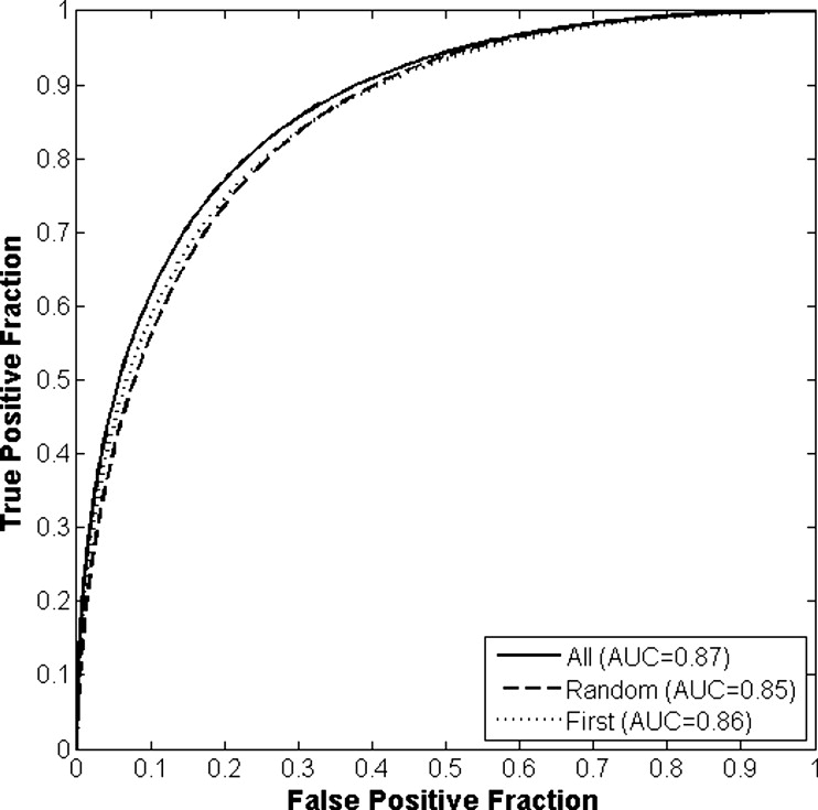
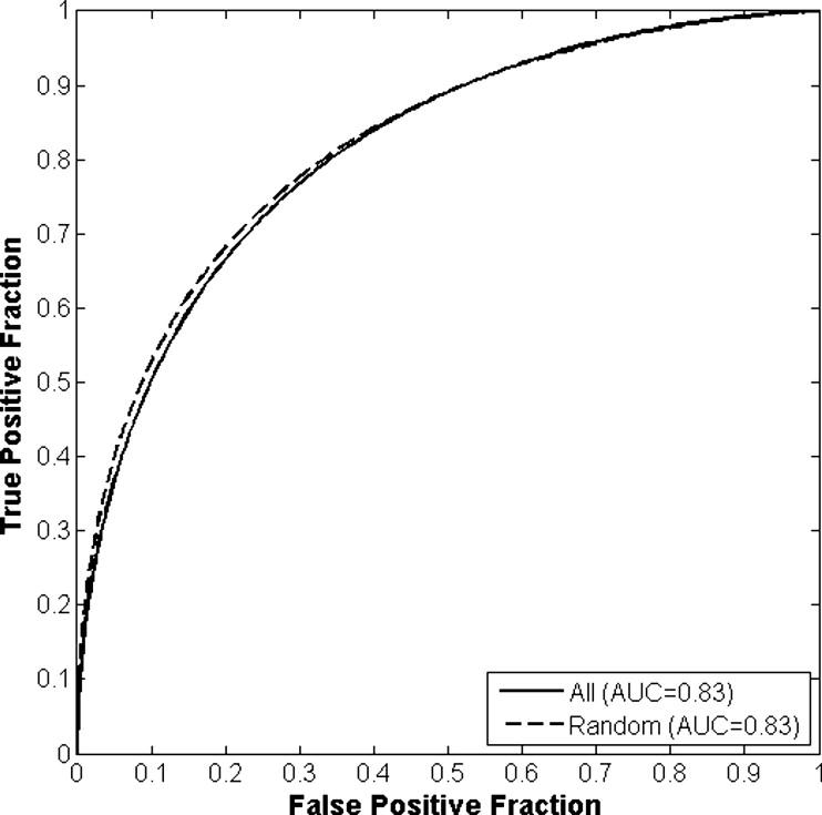
Table 2

Results of Round-robin Analyses for All Classification and View Selection Protocols Given as the Area Under the Receiver-Operating Characteristic Curve

View Protocol Classification Protocol A B C All images 0.86 (0.813–0.895) 0.87 (0.827–0.905) 0.83 (0.758–0.861) Random images 0.85 (0.806–0.889) 0.85 (0.810–0.892) 0.83 (0.745–0.870) First image only 0.86 (0.811–0.893) 0.86 (0.816–0.898) 0.86 (0.816–0.898)

Note: Data are indicated as area under the curve (two-sided 95% confidence interval).

Protocol A: Feature averaging; Protocol B: Classifier output averaging; Protocol C: No averaging.

Get Radiology Tree app to read full this article<

Table 3

Differences in Performance Between the View Selection Protocols for Each Classification Protocol

View Protocol Comparison Classification Protocol A B C All images vs. random images +0.01 (0.00 to 1) † +0.02 (0.00 to 0.04) ⁎ +0.00 (−0.02 to 1) † All images vs. first image only +0.00 (0.00 to 1) † +0.01 (0.00 to 1) † −0.04 (−0.08 to −0.01) ⁎ First image only vs. random images +0.01 (0.00 to 1) † +0.00 (0.00 to 1) † +0.04 (0.00 to 0.09) ⁎

Note: Data are indicated as difference in areas under the curves (95% confidence interval).

Protocol A: Feature averaging; Protocol B: Classifier output averaging; Protocol C: No averaging.

Get Radiology Tree app to read full this article<

Table 4

Differences in Performance Between the Classification Protocols for Each View Selection Protocol

View Protocol Classification Protocol Comparison B vs. A A vs. C B vs. C All images +0.01 (0.00–1) † +0.04 (0.01–0.09) ⁎ +0.05 (0.03–0.10) ⁎ Random images +0.00 (0.00–1) † +0.03 (0.00–0.09) ⁎ +0.03 (0.00–0.09) ⁎

Note: Data are indicated as difference in area under the curves (95% confidence interval).

Protocol A: Feature averaging; Protocol B: Classifier output averaging; Protocol C: No averaging.

Get Radiology Tree app to read full this article<

Discussion

Get Radiology Tree app to read full this article<

Appendix 1

Get Radiology Tree app to read full this article<

O=Area(C∩R)Area(C∪R), O

(

∩

)

(

∪

)

where O ranges from 0 to 1, with 0 representing no overlap and 1 representing a perfect match. The median value of the overlap was 0.924 with a 95% confidence interval of 0.922–0.927. The distribution of overlap values ( Fig 9 ) demonstrates that the seedpoint selected to begin automated segmentation has only a minimal effect on the segmentation process and that overall the process is fairly consistent. Instances of extremely low overlap ( O < 0.3) were often the result of random seedpoints that were as far from the center of the lesion as the constraints would allow, which is much less likely to occur if the user is instructed to place seedpoints on the center of the lesion (it is also less likely if the lesions are oddly shaped, as the lesion center becomes more “obvious” in those cases). If the random seedpoints are constrained to lie within a mask that has the same shape and centerpoint as the original lesion but only a quarter of its size, the median overlap improves to 0.943 (95% confidence interval, 0.941–0.945). Again this “quarter-size lesion mask” constraint is not unreasonable, as over time the user can be trained to place seedpoints as close to the center of a lesion as possible with minimal effort (using our observer data from above, radiologists placed seedpoints in this manner 93% (1313 of 1406) of the time). When comparing the values of the sonographic features extracted from the outlines, the average difference between the center seedpoint- and random seedpoint–generated outline feature values is nearly 0 for all four features ( Table 5 ). If the random seedpoints are constrained with a quarter-size mask instead of a half-size mask, the average feature differences remain consistent; only the average difference in the radial gradient index value decreased significantly ( P = .0001). Although the feature value standard deviations were not negligible, they seem to be small enough to conclude that overall the automated segmentation process is robust and can operate consistently with variations in input. However, we have also shown that it may be useful to pay more attention to seedpoint placement as the effect it might have is small but not necessarily irrelevant.

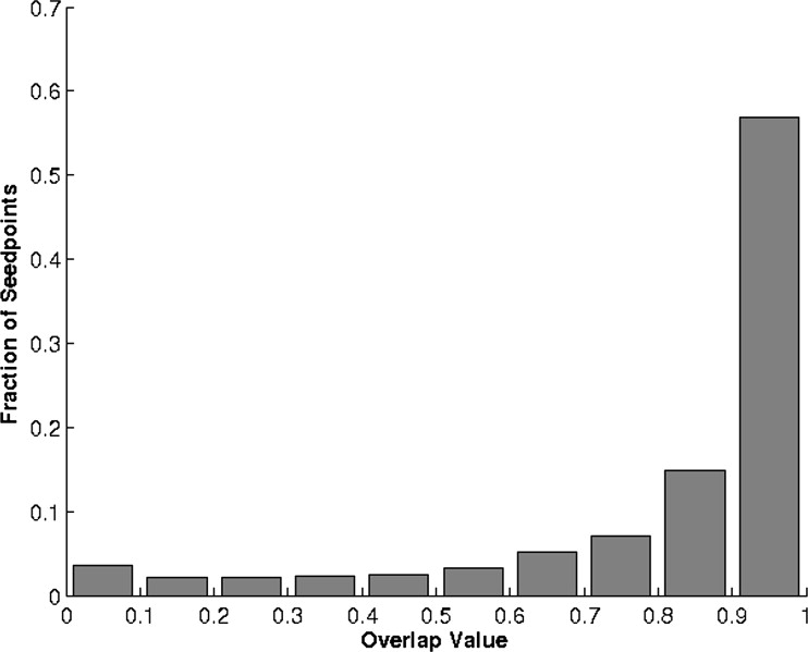
Table 5

Average Difference in Feature Values Between Outlines Generated Using the Center of the Lesion and Outlines Generated Using a Random Point Within the Lesion

Random Seedpoint Constraint Feature Difference D2W RGI MSD Corrl Mean SD Mean SD Mean SD Mean SD Quarter-size mask <0.001 0.053 0.001 0.085 −0.002 0.057 0.002 0.110 Half-size mask <0.001 0.060 0.005 0.098 −0.002 0.066 <0.001 0.120

Corrl: autocorrelation in depth direction (texture and shape); D2W: depth-to-width ratio (shape); MSD: maximum side difference (posterior acoustic behavior); RGI: radial gradient index (shape and sharpness).

Feature values have been normalized to between 0 and 1.

Get Radiology Tree app to read full this article<

Appendix 2

Get Radiology Tree app to read full this article<

References

1. Edwards B.K., Brown M.L., Wingo P.A., et. al.: Annual report to the nation on the status of cancer, 1975–2002, featuring population-based trends in cancer treatment. J Natl Cancer Inst 2005; 97: pp. 1407-1427.
2. Elmore J.G., Armstrong K., Lehman C.D., Fletcher S.W.: Screening for breast cancer. JAMA 2005; 293: pp. 1245-1256.
3. Fine R.E., Staren E.D.: Updates in breast ultrasound. Surg Clin North Am 2004; 84: pp. 1001-1034.
4. Kolb T.M.: Breast US for screening, diagnosing, and staging breast cancer: Issues and controversies; RSNA Categorical Course in Diagnostic Radiology Physics: Advances in Breast Imaging–Physics, Technology, and Clinical Applications 2004.2004.Radiologic Society of North AmericaChicago, IL ; 247–257
5. Berg W.A., Gutierrez L., NessAiver M.S., et. al.: Diagnostic accuracy of mammography, clinical examination, US, and MR imaging in preoperative assessment of breast cancer. Radiology 2004; 233: pp. 830-849.
6. Berg W.A., Blume J.D., Cormack J.B., Mendelson E.B., Madsen E.L., ACRIN 6666 Investigators: Lesion detection and characterization in a breast US phantom: Results of the ACRIN 6666 investigators. Radiology 2006; 239: pp. 693-702.
7. Jackson V.P.: The role of US in breast imaging. Radiology 1990; 177: pp. 305-311.
8. Sickles E.A.: Breast imaging: From 1965 to the present. Radiology 2000; 215: pp. 1-16.
9. Weinstein S.P., Conant E.F., Sehgal C.: Technical advances in breast ultrasound imaging. Semin Ultrasound CT MRI 2006; 27: pp. 273-283.
10. Horsch K., Giger M.L., Venta L.A., Vyborny C.J.: Computerized diagnosis of breast lesions on ultrasound. Med Phys 2002; 29: pp. 157-164.
11. Horsch K., Giger M.L., Vyborny C.J., Venta L.A.: Performance of computer-aided diagnosis in the interpretation of lesions on breast sonography. Acad Radiol 2004; 11: pp. 272-280.
12. Horsch K., Giger M.L., Vyborny C.J., Lan L., Mendelson E.B., Hendrick R.E.: Classification of breast lesions with multimodality computer-aided diagnosis: Observer study results on an independent clinical data set. Radiology 2006; 240: pp. 357-368.
13. Horsch K., Giger M.L., Venta L.A., Vyborny C.J.: Automatic segmentation of breast lesions on ultrasound. Med Phys 2001; 28: pp. 1652-1659.
14. Madjar H., Jellins J.: The Practice of Breast Ultrasound: Techniques, Findings, Differential Diagnosis.2000.ThiemeStuttgart/New York
15. Kupinski M.A., Edwards D.C., Giger M.L., Metz C.E.: Ideal observer approximation using Bayesian classification neural networks. IEEE Trans Med Imaging 2001; 20: pp. 886-899.
16. Metz C.E.: Fundamental ROC analysis.Beutel J.Kundel H.J.Van Metter R.L.Handbook of Medical Imaging, Volume 1: Physics and Psychophysics.2000.SPIE PressBellingham, WA:pp. 751-764.
17. Obuchowski N.A.: Receiver operating characteristic curves and their use in radiology. Radiology 2003; 229: pp. 3-8.
18. Pesce L.L., Metz C.E.: Proproc v2.2.0. Department of Radiology, University of Chicago. http://xray.bsd.uchicago.edu/krl/roc_soft.htm Updated February 27, 2007. Accessed July 1, 2007
19. Pesce L.L., Metz C.E.: Reliable and computationally efficient maximum-likelihood estimation of “proper” binormal ROC curves. Acad Radiol 2007; 14: pp. 814-829.
20. Pepe M.S.: The Statistical Evaluation of Medical Tests for Classification and Prediction.2004.Oxford University PressNew York
21. Mossman D.: Resampling techniques in the analysis of non-binormal ROC data. Med Decis Making 1995; 15: pp. 358-366.
22. Glantz S.A.: Primer of Biostatistics.6th ed2005.McGraw-HillNew York :219–251
23. Pocock S.J.: The pros and cons of noninferiority trials. Fundam Clin Pharmacol 2003; 17: pp. 483-490.
24. Piaggio G., Elbourne D.R., Altman D.G., Pocock S.J., Evans S.J.W.: Reporting of noninferiority and equivalence randomized trials: An extension of the CONSORT statement. JAMA 2006; 295: pp. 1152-1160.
25. Jenkins R., Burton A.M.: 100% accuracy in automatic face recognition. Science 2008; 319: pp. 435.
26. Huo Z., Giger M.L., Vyborny C.J.: Computerized analysis of multiple-mammographic views: Potential usefulness of special view mammograms in computer-aided diagnosis. IEEE Trans Med Imaging 2001; 20: pp. 1285-1292.
27. Liu B., Metz C.E., Jiang Y.: Effect of correlation on combining diagnostic information from two images of the same patient. Med Phys 2005; 32: pp. 3329-3338.
28. Metz C.E., Pan X.: “Proper” binormal ROC curves: Theory and maximum-likelihood estimation. J Math Psychol 1999; 43: pp. 1-33.

Performance of Breast Ultrasound Computer-aided Diagnosis

Rationale and Objectives

Materials and Methods

Results

Conclusion

Materials and Methods

Image Database

Image Selection Protocols

Lesion Classification Protocols

Performance Assessment and Statistical Analysis

Results

Discussion

Appendix 1

Appendix 2

References

Further Reading

Abstracts of Funded National Institutes of Health Grants

Accurate Automatic Papillary Muscle Identification for Quantitative Left Ventricle Mass Measurements in Cardiac Magnetic Resonance Imaging

All you need to know