
Rationale and Objectives
To assess the performance of dual-energy computed tomography (DECT) equipped with the new tin filter technology to classify phantom renal lesions as cysts or enhancing masses.
Materials and Methods
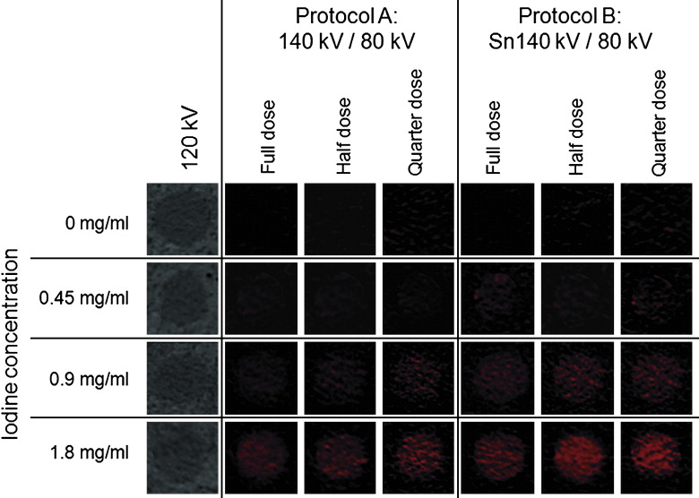
Forty spherical lesion proxies ranging in diameter from 6 to 27 mm were filled with either distilled water ( n = 10) representing cysts or titrated iodinated contrast solutions with a concentration of 0.45 ( n = 10), 0.9 ( n = 10), and 1.8 mg/mL ( n = 10) representing enhancing masses. The lesion proxies were placed in a 12-cm diameter renal phantom containing minced beef and submerged in a 28-cm water bath. DECT was performed using the new dual-source CT system (Definition Flash, Siemens Healthcare, Forchheim, Germany) allowing for an improved energy separation by using a tin filter. DECT was performed at tube voltages of 140/80 kV without the tin filter (protocol A) and with tin filter (protocol B). The tube current time product was selected in each protocol to achieve a constant CTDI (computed tomography dose index) with both protocols of 19 mGy (full dose), 9.5 mGy (half dose), and 4.8 mGy (quarter dose). Two blinded readers classified each lesion as a cyst or enhancing mass by using iodine overlay (IO) images. One reader measured the CT numbers of each lesion at 120 kV, in the IO, linear blending (LB), and virtual noncontrast (VNC) images.
Results
The CT numbers of the lesions at 120 kV were 0.1 ± 0.7 HU (0 mg iodine/mL), 9.1 ± 0.7 HU (0.45 mg/mL), 18.1 ± 1.4 HU (0.9 mg/mL), and 37.6 ± 1.6 HU (1.8 mg/mL). Mean diameter of the lesion proxies filled with water or different iodine concentrations was similar ( P = 0.38). Image noise was not significantly different in protocols A and B at the corresponding dose levels. At full dose, protocol A had a sensitivity of 93% and a specificity of 60% for discriminating renal lesions. Sensitivity and specificity declined to 84% and 38% at quarter dose. In protocol B, sensitivity was 100% and specificity was 90% at full dose and 93% and 70% at quarter dose. All misclassifications occurred in cyst or low iodine concentration (0.45 mg/mL) lesion proxies. The differences between CT numbers at 120 kV and in the IO, VNC, and AW (average weighted) images were significantly lower in protocol B compared to protocol A (each P < .05).
Conclusions
DECT using the tin filter results in an improved sensitivity and specificity for discriminating renal cysts from enhancing masses in a kidney phantom model and demonstrates higher dose efficiency as compared to former dual energy technology without tin filters.
The computed tomography (CT) discrimination of renal lesions bases on the presence of contrast enhancement during the nephrographic phase of contrast enhancement. For this reason, the standard practice in genitourinary CT includes both a noncontrast CT acquisition to assess baseline attenuation of renal masses as well as a contrast-enhanced CT acquisition to measure contrast enhancement within the mass.
Up to two thirds of all renal cell carcinomas are discovered incidentally during CT studies obtained for nonurological indications , and often only a contrast-enhanced CT data set but no noncontrast CT data is available. In few cases a renal lesion can be categorized as a solid lesion based on the presence of heterogeneous hyperattenuation on the contrast-enhanced CT data alone . However, in most instances, a hyperattenuating cyst may be difficult distinguished from a slightly enhancing renal cell carcinoma . In cases of incidentally discovered renal lesions, the patient has to be recalled to a complete genitourinary CT workup (including a noncontrast CT data acquisition) to establish the diagnosis.
Get Radiology Tree app to read full this article<
 Open full size image
Figure 1
Schematic drawing of the photon energy spectra of 80 kV tube voltage (- - -), 140 kV without tin filter (— — —), and 140 kV with tin filter (Sn140, ——). The tin filter increases energy separation by minimizing the overlap of high and low kVp spectra and reduces dose by blocking low energy photons from the high energy x-ray tube spectrum.
Get Radiology Tree app to read full this article<
Get Radiology Tree app to read full this article<
Materials and methods
Renal Phantom
Get Radiology Tree app to read full this article<
Renal Cyst and Attenuating Mass Proxies
Get Radiology Tree app to read full this article<
Experimental Setup
Get Radiology Tree app to read full this article<
Get Radiology Tree app to read full this article<
Get Radiology Tree app to read full this article<
Get Radiology Tree app to read full this article<
Table 1
Tube Voltage and Tube Current Settings in the Nine Dual-energy Computed Tomography Protocols
Tube A Tube B Protocol Tube voltage (kV) Tube current (mA) Tube voltage (kV) Tube current (mA) CTDI vol (mGy) A 140 70 80 385 18.8 A/2 140 35 80 193 9.6 A/4 140 17 80 94 4.7 B 80 430 Sn140 ∗ 233 19.0 B/2 80 215 Sn140 ∗ 116 9.5 B/4 80 108 Sn140 ∗ 58 4.8
CTDI vol , computed tomography dose index accounting the helical pitch or axial scan spacing
Get Radiology Tree app to read full this article<
Get Radiology Tree app to read full this article<
Get Radiology Tree app to read full this article<
Get Radiology Tree app to read full this article<
Get Radiology Tree app to read full this article<
Dual-energy Image Reconstruction
Get Radiology Tree app to read full this article<
Get Radiology Tree app to read full this article<
CT Data Analysis
Get Radiology Tree app to read full this article<
Get Radiology Tree app to read full this article<
Statistical Analysis
Get Radiology Tree app to read full this article<
Get Radiology Tree app to read full this article<
Get Radiology Tree app to read full this article<
Get Radiology Tree app to read full this article<
Get Radiology Tree app to read full this article<
Get Radiology Tree app to read full this article<
Results
Renal Lesion Characteristics
Get Radiology Tree app to read full this article<
Image Noise
Get Radiology Tree app to read full this article<
Quantitative Measurements in Lesion Proxies
Get Radiology Tree app to read full this article<
Table 2
CT Numbers in the Lesion Proxies Using the Different Dual-energy CT Protocols
Iodine Concentration Protocol A Protocol A/2 Protocol A/4 Protocol B Protocol B/2 Protocol B/4 0 mg/mL Weighted average images (HU) -0.4 ± 1.7 (-2.5 to 2.3) -0.3 ± 1.6 (-2.0 to 2.1) -0.9 ± 2.0 (-3.1 to 2.0) -0.1 ± 0.7 (-1.1 to 1.2) 0.1 ± 1.5 (-1.9 to 2.4) 0.3 ± 1.7 (6.7 to 12.2) Virtual noncontrast (HU) -1.2 ± 2.0 (-3.6 to 2.6) -1.1 ± 2.5 (-3.6 to 3.4) -1.4 ± 2.6 (-4.1 to 3.3) -0.2 ± 0.7 (-1.1 to 0.7) -0.2 ± 1.1 (-2.1 to 1.5) -0.1 ± 1.7 (-2.6 to 2.6) Subtracted iodine (HU) 0.8 ± 2.2 (-2.9 to 4.0) 1.3 ± 2.4 (-3.1 to 4.2) 0.6 ± 3.0 (-3.3 to 4.2) -0.1 ± 1.4 (-1.2 to 2.0) 0 ± 1.5 (-1.6 to 2.0) -0.2 ± 1.9 (-2.5 to 3.0) 0.45 mg/mL Weighted average images (HU) 8.3 ± 1.4 (6.1 to 10.3) 8.3 ± 1.4 (6.2 to 10.9) 8.2 ± 1.5 (6.3 to 10.2) 9.2 ± 0.6 (8.8 to 10.4) 9.3 ± 1.4 (7.4 to 12.3) 9.1 ± 1.7 (6.7 to 12.2) Virtual non contrast (HU) -1.6 ± 2.1 (-5.4 to 1.0) -1.1 ± 2.3 (-4.0 to 2.1) -0.9 ± 3.1 (-5.0 to 3.0) 0.2 ± 1.4 (-1.5 to 1.9) 0.2 ± 1.4 (-1.3 to 2.8) 0.2 ± 1.1 (-1.0 to 2.2) Subtracted iodine (HU) 10.2 ± 2.7 (6.4 to 15.0) 10.8 ± 2.9 (5.5 to 14.0) 10.9 ± 1.9 (8.8 to 14.4) 8.9 ± 0.8 (8.0 to 10.1) 9.3 ± 1.5 (7.0 to 12.3) 9.6 ± 2.1 (6.9 to 12.5) 0.9 mg/mL Weighted average images (HU) 17.2 ± 1.3 (15.2 to 19.8) 17.1 ± 1.5 (15.5 to 19.7) 17.0 ± 2.1 (13.8 to 20.3) 17.9 ± 1.0 (16.5 to 19.1) 17.1 ± 1.3 (15.1 to 19.5) 17.2 ± 1.9 (14.1 to 20.0) Virtual noncontrast (HU) -1.7 ± 3.3 (-6.2 to 3.8) -1.5 ± 3.4 (-5.4 to .1) -1.0 ± 3.8 (-5.8 to 5.5) 0.3 ± 1.0 (-0.5 to 1.6) -0.1 ± 1.1 (-2.5 to 1.4) 0.5 ± 1.5 (-1.9 to 2.5) Subtracted iodine (HU) 19.7 ± 1.9 (17.0 to 22.9) 19.5 ± 2.1 (16.0 to 22.5) 20.4 ± 2.8 (15.5 to 24.7) 17.8 ± 1.0 (16.5 to 19.2) 18.8 ± 1.7 (16.2 to 21.5) 18.9 ± 2.6 (15.1 to 22.3) 1.8 mg/mL Weighted average images (HU) 36.4 ± 1.8 (33.2 to 39.1) 36.1 ± 2.5 (32.5 to 39.1) 36.5 ± 2.2 (32.8 to 39.9) 37.7 ± 1.2 (35.6 to 38.5) 37.3 ± 1.4 (34.2 to 39.2) 37.0 ± 1.8 (33.6 to 39.9) Virtual noncontrast (HU) -1.2 ± 2.6 (-5.8 to 3.4) -1.0 ± 3.1 (-5.9 to 4.6) -1.3 ± 3.4 (-4.9 to 4.7) 0.2 ± 1.2 (-1.3 to 1.3) 0.1 ± 1.1 (-1.3 to 1.4) -0.1 ± 2.1 (-3.6 to 2.8) Subtracted iodine (HU) 38.2 ± 2.0 (34.9 to 41.2) 38.4 ± 1.7 (35.1 to 42.1) 38.4 ± 2.4 (35.1 to 42.1) 37.4 ± 0.6 (37.2 to 38.8) 37.7 ± 1.8 (33.7 to 40.9) 38.1 ± 1.6 (35.8 to 41.1)
CT, computed tomography; HU, Hounsfield units.
Get Radiology Tree app to read full this article<
Get Radiology Tree app to read full this article<
Get Radiology Tree app to read full this article<
Qualitative Interpretation of the Lesion Proxies
Get Radiology Tree app to read full this article<
Table 3
Diagnostic Performance of the Different Dual-energy Computed Tomography Protocols for Discrimination of Cysts and Renal Masses
Protocol A Protocol A/2 Protocol A/4 Protocol B Protocol B/2 Protocol B/4 True positives 28 27 27 30 29 28 True negatives 6 6 5 9 9 7 False positives 4 4 5 1 1 3 False negatives 2 3 3 0 1 2 Sensitivity [%] 93.3 (77.9–99.2) 81.8 (64.5–93.0) 84.4 (64.2–94.7) 100 (88.4–100) 96.7 (82.8–99.9) 93.3 (77.9–99.2) Specificity [%] 60.0 (26.2–87.8) 42.9 (9.9–81.6) 37.5 (8.5–75.5) 90.0 (55.5–99.8) 90.0 (55.5–99.8) 70.0 (34.8–93.3)
Get Radiology Tree app to read full this article<
Get Radiology Tree app to read full this article<
Get Radiology Tree app to read full this article<
Get Radiology Tree app to read full this article<
Discussion
Get Radiology Tree app to read full this article<
Get Radiology Tree app to read full this article<
Get Radiology Tree app to read full this article<
Get Radiology Tree app to read full this article<
Get Radiology Tree app to read full this article<
Get Radiology Tree app to read full this article<
Get Radiology Tree app to read full this article<
Get Radiology Tree app to read full this article<
Get Radiology Tree app to read full this article<
Get Radiology Tree app to read full this article<
Get Radiology Tree app to read full this article<
References
1. Volpe A., Panzarella T., Rendon R.A., et. al.: The natural history of incidentally detected small renal masses. Cancer 2004; 100: pp. 738-745.
2. Brown C.L., Hartman R.P., Dzyubak O.P., et. al.: Dual-energy CT iodine overlay technique for characterization of renal masses as cyst or solid: a phantom feasibility study. Eur Radiol 2009; 19: pp. 1289-1295.
3. Millner M.R., McDavid W.D., Waggener R.G., et. al.: Extraction of information from CT scans at different energies. Med Phys 1979; 6: pp. 70-71.
4. Chandarana H., Godoy M.C., Vlahos I., et. al.: Abdominal aorta: evaluation with dual-source dual-energy multidetector CT after endovascular repair of aneurysms—initial observations. Radiology 2008; 249: pp. 692-700.
5. Fletcher J.G., Takahashi N., Hartman R., et. al.: Dual-energy and dual-source CT: is there a role in the abdomen and pelvis?. Radiol Clin North Am 2009; 47: pp. 41-57.
6. Graser A., Johnson T.R., Bader M., et. al.: Dual energy CT characterization of urinary calculi: initial in vitro and clinical experience. Invest Radiol 2008; 43: pp. 112-119.
7. Graser A., Johnson T.R., Chandarana H., et. al.: Dual energy CT: preliminary observations and potential clinical applications in the abdomen. Eur Radiol 2009; 19: pp. 13-23.
8. Primak A.N., Ramirez Giraldo J.C., et. al.: Improved dual-energy material discrimination for dual-source CT by means of additional spectral filtration. Med Phys 2009; 36: pp. 1359-1369.
9. Scheffel H., Stolzmann P., Frauenfelder T., et. al.: Dual-energy contrast-enhanced computed tomography for the detection of urinary stone disease. Invest Radiol 2007; 42: pp. 823-829.
10. Stolzmann P., Frauenfelder T., Pfammatter T., et. al.: Endoleaks after endovascular abdominal aortic aneurysm repair: detection with dual-energy dual-source CT. Radiology 2008; 249: pp. 682-691.
11. Stolzmann P., Scheffel H., Rentsch K., et. al.: Dual-energy computed tomography for the differentiation of uric acid stones: ex vivo performance evaluation. Urol Res 2008; 36: pp. 133-138.
12. Brodoefel H., Burgstahler C., Heuschmid M., et. al.: Accuracy of dual-source CT in the characterization of non-calcified plaque: use of a colour-coded analysis compared with virtual histology intravascular ultrasound. Br J Radiol 2009; 82: pp. 805-812.
13. Landis J.R., Koch G.G.: The measurement of observer agreement for categorical data. Biometrics 1977; 33: pp. 159-174.
14. Duchene D.A., Lotan Y., Cadeddu J.A., et. al.: Histopathology of surgically managed renal tumors: analysis of a contemporary series. Urology 2003; 62: pp. 827-830.
15. Jinzaki M., Tanimoto A., Mukai M., et. al.: Double-phase helical CT of small renal parenchymal neoplasms: correlation with pathologic findings and tumor angiogenesis. J Comput Assist Tomogr 2000; 24: pp. 835-842.