
Rationale and Objectives
To more reliably recover cardiac information from noise-corrupted, patient-specific measurements, it is essential to employ meaningful constraining models and adopt appropriate optimization criteria to couple the models with the measurements. Although biomechanical models have been extensively used for myocardial motion recovery with encouraging results, the passive nature of such constraints limits their ability to fully count for the deformation caused by active forces of the myocytes. To overcome such limitations, we propose to adopt a cardiac physiome model as the prior constraint for cardiac motion analysis.
Materials and Methods
The cardiac physiome model comprises an electric wave propagation model, an electromechanical coupling model, and a biomechanical model, which are connected through a cardiac system dynamics for a more complete description of the macroscopic cardiac physiology. Embedded within a multiframe state-space framework, the uncertainties of the model and the patient’s measurements are systematically dealt with to arrive at optimal cardiac kinematic estimates and possibly beyond.
Results
Experiments have been conducted to compare our proposed cardiac-physiome–model-based framework with the solely biomechanical model-based framework. The results show that our proposed framework recovers more accurate cardiac deformation from synthetic data and obtains more sensible estimates from real magnetic resonance image sequences.
Conclusion
With the active components introduced by the cardiac physiome model, cardiac deformations recovered from patient’s medical images are more physiologically plausible.
The goal of computational cardiac analysis is to objectively and accurately recover parameters of various cardiac functions based on specific measurements on patients, such as those obtained from medical imaging, electrocardiograms, and blood pressures ( ). Nevertheless, these noninvasive measurements and in vivo measurements can only provide either sparse, or gross, or projective observations in spatial or temporal domains, and are usually corrupted by noises of various sources. As a result, analysis based solely on measurements is ill-posed, and thus models obtained from invasive or in vitro experiments, such as those from anatomy, biomechanics, or physiology, are necessary to relate the measurements with the cardiac parameters of interest to properly formulate the inverse problems.
Cardiac Physiome Model and Patient’s Measurements
At the beginning of each cardiac cycle, pacemaker cells in the heart generate action potentials that are conducted to the whole heart through conduction fibers, including the atrioventricular bundle located in the interventricular septum, the left and the right bundle branches that conduct impulses to the left and the right ventricles, and the Purkinje fibers that spread throughout the ventricular myocardium ( ). The myocardial contractile cells are excited by the action potentials, contract according to the sequence of excitations, and the heart beats in a rhythmic motion. Thus, to properly model the cyclic motion of the heart, the cardiac electric wave propagation model (E model) ( ), the electromechanical coupling model (EM model) ( ), and the myocardial biomechanical model (BM model) ( ) are required. The E model describes the spatiotemporal propagation pattern of the action potentials, providing the excitation sequence of the myocytes. The excitations are then transformed into contraction stresses by the EM model, providing the myocardium contraction forces, which deform the heart according to the mechanical properties governed by the BM model through the cardiac system dynamics. Because the combination of these three models gives a relatively complete description of the macroscopic physiologic behavior of the heart, it is termed the cardiac physiome model . Several experiments have been done on the simulations of the heart cycle using the cardiac physiome model and validated through different criteria ( ), which shows that the cardiac physiome model provides a useful tool for analyzing cardiac physiology and pathology.
Get Radiology Tree app to read full this article<
Computational Cardiac Information Recovery
Get Radiology Tree app to read full this article<
Get Radiology Tree app to read full this article<
Contributions
Get Radiology Tree app to read full this article<
Materials and methods
Get Radiology Tree app to read full this article<
Electric Wave Propagation Model
Get Radiology Tree app to read full this article<
∂u∂t=∇⋅(D∇u)+c1u(u−a)(1−u)−c2uv∂v∂t=b(u−dv) ∂
u
∂
t
=
∇
⋅
(
D
∇
u
)
+
c
1
u
(
u
−
a
)
(
1
−
u
)
−
c
2
u
v
∂
v
∂
t
=
b
(
u
−
d
v
)
where u is the transmembrane potential, v is the recovery variable, D is the diffusion tensor, and a , b , c 1 , c 2 , and d are parameters that define the shape of the action potential. These parameters are constant in time but not necessarily in space. The diffusion tensor D is related to the fiber orientation, which is defined under a global cartesian coordinate system. Under the local fiber coordinate system, in which the x-axis aligns with the fiber, the local diffusion tensor D local can be defined as:
Dlocal=⎡⎣⎢⎢df000dcf000dcf⎤⎦⎥⎥ D
local
=
[
d
f
0
0
0
d
c
f
0
0
0
d
c
f
]
where d f and d cf are the diffusion tensor coefficients along the fiber and cross the fiber, respectively. d f is usually four times larger than d cf , so that the action potential propagates faster along the fiber direction. D local can then be transformed into D using tensor transformation with the fiber orientation considered ( ).
Get Radiology Tree app to read full this article<
Get Radiology Tree app to read full this article<
Electromechanical Coupling Model
Get Radiology Tree app to read full this article<
∂σc∂t+σc=uσ0 ∂
σ
c
∂
t
+
σ
c
=
u
σ
0
where σ c is a scalar related to the stress tensor, and σ 0 is a constant for scaling the stress.
Get Radiology Tree app to read full this article<
Get Radiology Tree app to read full this article<
{σc(t)=σ0(1−eαc(Td−t)),ifTd≤t≤Trσc(t)=σreαr(Tr−t)),ifTr≤t≤Td+HP {
σ
c
(
t
)
=
σ
0
(
1
−
e
α
c
(
T
d
−
t
)
)
,
i
f
T
d
≤
t
≤
T
r
σ
c
(
t
)
=
σ
r
e
α
r
(
T
r
−
t
)
)
,
i
f
T
r
≤
t
≤
T
d
+
H
P
where T d and T r are the depolarization time and the repolarization time, respectively, which are determined according to the temporal pattern of u . HP is the heart period, α c is the contraction rate, α r is the relaxation rate, and σ r = σ c ( T r ). α c and α r are introduced for better control of the increase and decrease of the contraction stress; a time constant can also be added to T d and T r to model the delay between the electrical and the mechanical phenomena.
Get Radiology Tree app to read full this article<
Get Radiology Tree app to read full this article<
σ=−σcf⊗f σ
=
−
σ
c
f
⊗
f
with f the fiber orientation vector under the current configuration of the heart geometry and ⊗ the tensor product. The minus sign is necessary because σ c is always positive while a contraction tensor is required. Thus σ is a Cauchy stress tensor defined under the deformed configuration. Because the total-Lagrangian cardiac system dynamic is used in our framework in which forces defined under the reference configuration are required, σ is transformed into the first Piola-Kirchhoff stress tensor through
P=Jσ(F−1)T P
=
J
σ
(
F
−
1
)
T
where F is the deformation gradient and J = det (F) .
Get Radiology Tree app to read full this article<
Get Radiology Tree app to read full this article<
Rbody=−Div(P)=−Jdiv(σ)=Jdiv(σcf⊗f) R
b
o
d
y
=
−
Div
(
P
)
=
−
J
div
(
σ
)
=
J
div
(
σ
c
f
⊗
f
)
with Div( · ) and div( · ) the divergence operators with respect to the material and the spatial coordinate systems, respectively. The active surface force per unit area in the reference configuration can be obtained as:
Rsurface=PN R
s
u
r
f
a
c
e
=
PN
where N is the outward surface normal in the reference configuration. These active contraction forces R body and R surface can then be integrated into the cardiac system dynamics using mesh-free methods ( ).
Get Radiology Tree app to read full this article<
Biomechanical Model
Get Radiology Tree app to read full this article<
Get Radiology Tree app to read full this article<
S=Cϵ S
=
C
ϵ
where S = [S 11 S 22 S 33 S 12 S 13 S 23 ] T and ϵ = [ϵ 11 ϵ 22 ϵ 33 ϵ 12 ϵ 13 ϵ 23 ] T , with S ij the components of the second Piola-Kirchhoff stress tensor and ϵ ij the components of the Green-Lagrangian strain tensor, which are defined under a cartesian coordinate system ( x, y, z ) in our current framework. C is the stiffness matrix containing the material properties. According to the literature ( ), the structure and composition of the heart are very complicated. In the macroscopic view, the myocardium can be treated as a composite material, a continuous constituent of collagen tissues reinforced by myofibers ( ). Because the Young’s moduli for a composite material with fibrous reinforcements are different along and across the fibers, the myocardium is anisotropic in nature. Because the myofibers are tubular in shape, and mechanical testings have shown that the material properties of the transverse planes along a myofiber are nearly isotropic ( ), the myofibers are thus modeled as transversely isotropic materials in our work. Let C o be the three-dimensional stiffness matrix of a point in the myocardium under the local fiber coordinate system:
Co=⎡⎣⎢⎢⎢⎢⎢⎢⎢⎢⎢⎢⎢⎢⎢⎢1Ef−vfEcf−vfEcf000−vfEcf1Ecf−vcfEcf000−vfEcf−vcfEcf1Ecf0000001G0000001G0000002(1+vcf)Ecf⎤⎦⎥⎥⎥⎥⎥⎥⎥⎥⎥⎥⎥⎥⎥⎥−1 C
o
=
[
1
E
f
−
v
f
E
c
f
−
v
f
E
c
f
0
0
0
−
v
f
E
c
f
1
E
c
f
−
v
c
f
E
c
f
0
0
0
−
v
f
E
c
f
−
v
c
f
E
c
f
1
E
c
f
0
0
0
0
0
0
1
G
0
0
0
0
0
0
1
G
0
0
0
0
0
0
2
(
1
+
v
c
f
)
E
cf
]
−
1
E f , E cf , v f , v cf are the Young’s moduli and Poisson’s ratios along and cross the fiber, respectively, G ≈ E f /(2(1 + v f )) describes the shearing property. (If E f = E cf and v f = v cf , then C o reduces to the stiffness matrix for isotropic materials.)
Get Radiology Tree app to read full this article<
Get Radiology Tree app to read full this article<
C=T−1CoRTR−1 C
=
T
−
1
C
o
R
T
R
−
1
where T is a tensor transformation matrix related to the fiber orientation, and R is a diagonal matrix responsible for the transformation between the strain tensor components and the engineering strain tensor components ( ). The symmetry of C o is inherited to C after the tensor transformation.
Get Radiology Tree app to read full this article<
Cardiac System Dynamics Under Finite Deformation
Get Radiology Tree app to read full this article<
M0tU¨t+△t+C0tU˙t+△t+K˜0tΔU=Rct+△t+Rbt+△t−Ri0t M
0
t
U
¨
t+
△
t
+
C
0
t
U
˙
t+
△
t
+
K
˜
0
t
Δ
U=
R
c
t+
△
t
+
R
b
t+
△
t
−
R
i
0
t
where M0t M
0
t is the mass matrix, C0t C
0
t is the damping matrix, and K˜0t K
˜
0
t is the strain incremental stiffness matrix that contains the internal stresses and the material and deformation properties at time t . t+Δt R c is the force vector containing the contractile active forces R body and R surface in Eq 7 and Eq 8 , produced by the E and EM models. t+Δt R b is the force vector for enforcing boundary conditions, and R0ti R
0
t
i is the nodal force vector for finite deformation only and is related to the internal stresses at time t . U¨t+△t U
¨
t+
△
t , U˙t+△t U
˙
t+
△
t , and Δ U are the respective nodal acceleration, velocity, and incremental displacement vectors at time t + Δ t .
Get Radiology Tree app to read full this article<
Get Radiology Tree app to read full this article<
Optimal Multiframe Kinematic Estimation: Coupling of Cardiac Physiome Model and Patient’s Measurements
Get Radiology Tree app to read full this article<
Get Radiology Tree app to read full this article<
x(t+Δt)=F(t)x(t)+w(t+Δt) x
(
t
+
Δ
t
)
=
F
(
t
)
x
(
t
)
+
w
(
t
+
Δ
t
)
where x ( t +Δ t ) = t+Δt U and x(t) = t U are the state vectors, containing the nodal displacements at time t and ( t +Δ t ), the kinematic quantities we want to recover. F(t) is the transition matrix relating x ( t +Δ t ) with x ( t) , and is composed of the M0t M
0
t , C0t C
0
t , and K˜0t K
˜
0
t matrices of Eq 11 . w(t+ Δ t) is the input vector that contains the force inputs of the right side of Eq 11 , including the contractile force vector t+Δt R c obtained from the cardiac physiome model. Considering also the zero-mean, additive, and white system uncertainties, v(t)(E[v(t)]=0,E[v(t)v(s)’]=Qv(t)δts v
(
t
)
(
E
[
v
(
t
)
]
=
0
,
E
[
v
(
t
)
v
(
s
)
′
]
=
Q
v
(
t
)
δ
t
s Eq 12 becomes a total Lagrangian–updated state-space equation that performs nonlinear state prediction (displacement) using the Newton-Raphson iteration scheme:
x(t+Δt)=F(t)x(t)+w(t+Δt)+v(t+Δt) x
(
t
+
Δ
t
)
=
F
(
t
)
x
(
t
)
+
w
(
t
+
Δ
t
)
+
v
(
t
+
Δ
t
)
and x ( t+Δt ) becomes a statistical representation with system uncertainties.
Get Radiology Tree app to read full this article<
Get Radiology Tree app to read full this article<
y(t+Δt)=Hx(t+Δt)+e(t+Δt) y
(
t
+
Δ
t
)
=
H
x
(
t
+
Δ
t
)
+
e
(
t
+
Δ
t
)
where y ( t+Δt ) contains the image-derived, patient-specific displacements, and H is a measurement matrix containing only 0 and 1 for the mapping between x ( t+Δt ) and y ( t+Δt ). With these statistical state-space Eq 13 and 14 defined, the active stresses, the cardiac deformation, and the patient measurements are connected. Using the multiframe filtering procedure described elsewhere ( ), the prior cardiac physiome kinematic predictions can be updated by the measurements to provide the optimal patient-specific estimates xˆ(t) x
(
t
) . (The real and perfect state x ( t ) is theoretically impossible to recover, thus what we can obtain is its estimate xˆ(t) x
(
t
) .) The procedure includes:
Get Radiology Tree app to read full this article<
Get Radiology Tree app to read full this article<
Get Radiology Tree app to read full this article<
xˆ−(t+Δt)=F(t)xˆ(t)+w(t+Δt) x
−
(
t
+
Δ
t
)
=
F
(
t
)
x
(
t
)
+
w
(
t
+
Δ
t
)
P−(t+Δt)=F(t)P(t)F(t)T+Qv(t) P
−
(
t
+
Δ
t
)
=
F
(
t
)
P
(
t
)
F
(
t
)
T
+
Q
v
(
t
)
3. Correction step: with the use of the Kalman gain G(t+Δt) , the predictions are updated using the measurements y(t+Δt) :
G(t+Δt)=P−(t+Δt)HT(HP−(t+Δt)HT+Re(t+Δt))−1 G
(
t
+
Δ
t
)
=
P
−
(
t
+
Δ
t
)
H
T
(
H
P
−
(
t
+
Δ
t
)
H
T
+
R
e
(
t
+
Δ
t
)
)
−
1
xˆ(t+Δt)=xˆ−(t+Δt)+G(t+Δt)(y(t+Δt)−Hxˆ−(t+Δt)) x
(
t
+
Δ
t
)
=
x
−
(
t
+
Δ
t
)
+
G
(
t
+
Δ
t
)
(
y
(
t
+
Δ
t
)
−
H
x
−
(
t
+
Δ
t
)
)
P(t+Δt)=(I−G(t+Δt)H)P−(t+Δt) P
(
t
+
Δ
t
)
=
(
I
−
G
(
t
+
Δ
t
)
H
)
P
−
(
t
+
Δ
t
)
In brief, P(t) and xˆ(t) x
(
t
) are first projected to time t+Δt using F(t) to obtain the predictions. Then the Kalman gain G(t+Δt ), which is used to update the predictions, is calculated based on Q v (t+Δt) , R e (t+Δt) and H , thus it can provide the optimal update in the minimum-mean squared-error sense based on the information of the system uncertainties and observation errors. With the aid of the Kalman gain, the estimate xˆ(t+Δt) x
(
t
+
Δ
t
) can be obtained through coupling the state prediction with measurement y(t+Δt) . The same procedure is applied to the consecutive frames to recover patient’s cardiac deformation for the whole cardiac cycle.
Get Radiology Tree app to read full this article<
Results
Get Radiology Tree app to read full this article<
Synthetic Data
Get Radiology Tree app to read full this article<
Get Radiology Tree app to read full this article<
Get Radiology Tree app to read full this article<
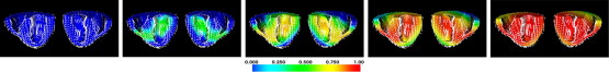
| 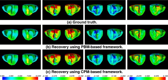 |
Get Radiology Tree app to read full this article<
Get Radiology Tree app to read full this article<
Table 1
Deviations of the Recovered Displacement Magnitudes (| u |) and Strains (ε αβ ) Against the Ground Truth
PBM-based CPM-based |u| (mm) 0.2705 ± 0.3636 0.2871 ± 0.4572 ϵ rr 0.0309 ± 0.0885 0.0198 ± 0.0322 ϵ θθ 0.0175 ± 0.0322 0.0159 ± 0.0276 ϵ zz 0.0205 ± 0.0531 0.0168 ± 0.0578 ϵ rθ 0.0176 ± 0.0420 0.0132 ± 0.0215 ϵ θz 0.0131 ± 0.0248 0.0113 ± 0.0181 ϵ zr 0.0175 ± 0.0474 0.0124 ± 0.0208
Strains are calculated under a cylindrical coordinate system ( r,θ,z ), with the long axis of the left ventricle as the z -axis.
PBM: passive-biomechanical model–based; CPM: cardiac-physiome-model–based.
Get Radiology Tree app to read full this article<
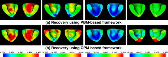
MR Image Data
Get Radiology Tree app to read full this article<
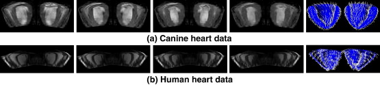
Get Radiology Tree app to read full this article<
Get Radiology Tree app to read full this article<
Get Radiology Tree app to read full this article<
|  |
| 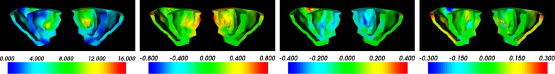 |
Get Radiology Tree app to read full this article<
Discussion
Get Radiology Tree app to read full this article<
Get Radiology Tree app to read full this article<
Get Radiology Tree app to read full this article<
References
1. Braunwald E.Zipes D.P.Libby P.Heart disease: a textbook of cardiovascular medicine.2001.W.B. Saunders CompanyPhiladelphia:
2. Germann W.J., Stanfield C.L.: Principles of human physiology.2005.Pearson Benjamin CummingsSan Francisco
3. Aliev R.R., Panfilov A.V.: A simple two-variable model of cardiac excitation. Chaos Solutions Fractals 1996; 7: pp. 293-301.
4. Knudsen Z., Holden A., Brindley J.: Qualitative modelling of mechano-electrical feedback in a ventricular cell. Bull Math Biol 1997; 6: pp. 115-181.
5. Hunter P., Smaill B.: The analysis of cardiac function: a continuum approach. Prog Biophys Molec Biol 1988; 52: pp. 101-164.
6. Nash M.: Mechanics and material properties of the heart using an anatomically accurate mathematical model.1998.University of Auckland
7. Fung Y.C.: Biomechanics: mechanical properties of living tissues.2nd ed.1993.Springer-VerlagNew York
8. Glass L.Hunter P.McCulloch Theory of heart: biomechanics, biophysics, and nonlinear dynamics of cardiac function.1991.Springer-VerlagNew York: 4
9. Hunter P.J., Borg T.K.: Integration from proteins to organs: the physiome project. Nat Rev Molec Cell Biol 2003; 4: pp. 237-243.
10. Sermesant M., Delingette H., Ayache N.: An electromechanical model of the heart for image analysis and simulation. IEEE Trans Med Imaging 2006; 25: pp. 612-625.
11. Frangi A.J., Niessen W.J., Viergever M.A.: Three-dimensional modeling for functional analysis of cardiac images: A review. IEEE Trans Med Imaging 2001; 20: pp. 2-25.
12. He B., Li G., Zhang X.: Noninvasive imaging of cardiac transmembrane potentials within three-dimensional myocardium by means of a realistic geometry anisotropic heart model. IEEE Trans Biomed Eng 2003; 50: pp. 1190-1202.
13. Wang L., Zhang H., Shi P., et. al.: Imaging of 3D cardiac electrical activity: a model-based recovery framework. Int Conf Med Image Computing Comp Assisted Intervention 2006; 4190: pp. 792-799.
14. Hu Z., Metaxas D., Axel L.: In vivo strain and stress estimation of the heart left and right ventricles from MRI images. Med Image Anal 2003; 7: pp. 435-444.
15. Shi P., Liu H.: Stochastic finite element framework for simultaneous estimation of cardiac kinematic functions and material parameters. Med Image Anal 2003; 7: pp. 445-464.
16. Liu H., Shi P.: Meshfree representation and computation: applications to cardiac motion analysis. Information Proc Med Imaging 2003; 2732: pp. 560-572.
17. Wong A., Liu H., Sinusas A., et. al.: Simultaneous recovery of left ventricular shape and motion using meshfree particle framework.IEEE Int Symp Biomed Imaging: Macro to Nano.2004.pp. 1263-1266.
18. Wong K.C.L., Shi P.: Finite deformation guided nonlinear filtering for multiframe cardiac motion analysis. Int Conf Med Image Computing Comp Assisted Intervention 2004; 3216: pp. 895-902.
19. Wong L.N., Liu H., Sinusas A., et. al.: Spatio-temporal active region model for simultaneous segmentation and motion estimation of the whole heart.IEEE Workshop on Variational, Geometric and Level Set Methods in Computer Vision.2003.pp. 193-200.
20. Rogers J.M., McCulloch A.D.: A collocation-Galerkin finite element model of cardiac action potential propagation. IEEE Trans Biomed Engineering 1994; 41: pp. 743-757.
21. Bathe K.J.: Finite element procedures.1996.Prentice HallEnglewood Cliffs, NJ
22. Liu G.R.: Mesh free methods: moving beyond the finite element method.2003.CRC PressBoca Raton, Fla
23. Hsu E.W., Henriquez C.S.: Myocardial fiber orientation mapping using reduced encoding diffusion tensor imaging. J Cardiovasc Magnet Res 2001; 3: pp. 339-347.
24. Zhang H., Shi P.: A meshfree method for solving cardiac electrical propagation.27th Annual International Conference of the IEEE-EMBS.2005.pp. 349-352.
25. Bestel J., Clement F., Sorine M.: A biomechanical model of muscle contraction. Conf Med Image Computing Comp Assisted Intervention 2001; 2208: pp. 1159-1161.
26. Holzapfel G.A.: Nonlinear solid mechanics: a continuum approach for engineering.2000.John Wiley & Sons, IncChichester
27. Matthews F.L., Rawlings R.D.: Composite materials: engineering and science.1994.Chapman & HallLondon
28. Besl P.J., McKay H.D.: A method for registration of 3-D shapes. IEEE Trans Pattern Anal Machine Intell 1992; 14: pp. 239-256.
29. Zhang H., Wong C.L., Shi P.: An inverse recovery of cardiac electrical propagation from image sequences. Med Imaging Augmented Reality 2006; 4091: pp. 132-139.
30. Moreau-Villéger V., Delingette H., Sermesant M., et. al.: Building maps of local apparent conductivity of the epicardium with a 2-D electrophysiological model of the heart. IEEE Trans Biomed Engineering 2006; 53: pp. 1457-1466.