
Rationale and Objectives
Perturbations in cerebral blood volume (CBV), blood flow (CBF), and metabolic rate of oxygen (CMRO 2 ) lead to associated changes in tissue concentrations of oxy- and deoxy-hemoglobin (Δ O and Δ D ), which can be measured by near-infrared spectroscopy (NIRS). A novel hemodynamic model has been introduced to relate physiological perturbations and measured quantities. We seek to use this model to determine functional traces of cbv( t ) and cbf( t ) − cmro 2 ( t ) from time-varying NIRS data, and cerebrovascular physiological parameters from oscillatory NIRS data (lowercase letters denote the relative changes in CBV, CBF, and CMRO 2 with respect to baseline). Such a practical implementation of a quantitative hemodynamic model is an important step toward the clinical translation of NIRS.
Materials and Methods
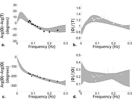
In the time domain, we have simulated O ( t ) and D ( t ) traces induced by cerebral activation. In the frequency domain, we have performed a new analysis of frequency-resolved measurements of cerebral hemodynamic oscillations during a paced breathing paradigm.
Results
We have demonstrated that cbv( t ) and cbf( t ) − cmro 2 ( t ) can be reliably obtained from O ( t ) and D ( t ) using the model, and that the functional NIRS signals are delayed with respect to cbf( t ) − cmro 2 ( t ) as a result of the blood transit time in the microvasculature. In the frequency domain, we have identified physiological parameters (e.g., blood transit time, cutoff frequency of autoregulation) that can be measured by frequency-resolved measurements of hemodynamic oscillations.
Conclusions
The ability to perform noninvasive measurements of cerebrovascular parameters has far-reaching clinical implications. Functional brain studies rely on measurements of CBV, CBF, and CMRO 2 , whereas the diagnosis and assessment of neurovascular disorders, traumatic brain injury, and stroke would benefit from measurements of local cerebral hemodynamics and autoregulation.
Near-infrared spectroscopy (NIRS) can assess noninvasively cerebral hemodynamics and brain function by being sensitive to cerebral concentrations of deoxyhemoglobin ( D ) and oxy-hemoglobin ( O ). Noninvasive measurements of task-related functional activity with NIRS, or fNIRS, have been reported . These hemodynamic changes result from changes in the cerebral blood volume (CBV), cerebral blood flow (CBF), and metabolic rate of oxygen (CMRO 2 ) as a result of brain activation and neurovascular coupling. Understanding the interplay between these physiological/functional/metabolic processes and the measured signals with functional neuroimaging techniques such as fNIRS and functional magnetic resonance imaging is the major objective of hemodynamic models (for a review, see Buxton, 2012 ).
A novel hemodynamic model has been recently introduced to provide an analytical tool for the study of oscillatory (frequency domain) and time varying (time domain) hemodynamics that are measurable with NIRS . The model relates normalized perturbations in CBV, CBF, and CMRO 2 to the dynamics of O and D concentrations in tissue. In particular, this model treats the cerebral microvasculature in terms of three compartments (arterial, capillary, venous) and describes the effects of changes in blood volume in all three compartments (even though the capillary contribution to blood volume changes may be negligible), and the effects of changes in blood flow and metabolic rate of oxygen in the capillary compartment (direct effects) and the venous compartment (indirect effects). This novel model can be applied to measurements in the time domain ( O ( t ), D ( t )), where hemodynamic changes are induced over time, and in the frequency domain (via the phasors O (ω), D (ω)), where induced hemodynamic oscillations are measured as a function of the frequency of oscillation. Hemodynamic oscillations at a specific frequency can be induced by a number of protocols including paced breathing , head-up-tilting , squat-stand maneuvers , and pneumatic thigh-cuff inflation , leading to a technique that we have recently proposed, coherent hemodynamics spectroscopy (CHS) .
Get Radiology Tree app to read full this article<
Get Radiology Tree app to read full this article<
. In the frequency domain, we demonstrate how the model can be used to measure a number of physiologically relevant parameters such as the blood transit time in the microvasculature and the cutoff frequency for cerebral autoregulation. The work presented here demonstrates, in practical terms, that the new hemodynamic model is a workable model for translation of NIRS measurements into functional and physiological parameters. The feasibility of a practical implementation of this mathematical model, in combination with noninvasive NIRS and fNIRS measurements, is a critical element for its translation toward functional and clinical studies.
Get Radiology Tree app to read full this article<
Hemodynamic model
Get Radiology Tree app to read full this article<
Time domain equations
Get Radiology Tree app to read full this article<
O(t)=ctHb[S(a)CBV(a)0(1+cbv(a)(t))+<S(c)>Ƒ(c)CBV(c)0+S(v)CBV(v)0(1+cbv(v)(t))]++ctHb[<S(c)>S(v)(<S(c)>−S(v))Ƒ(c)CBV(c)0h(c)RC−LP(t)+(S(a)−S(v))CBV(v)0h(v)G−LP(t)]∗[cbf(t)−cmro2(t)], O
(
t
)
=
ctHb
[
S
(
a
)
CBV
0
(
a
)
(
1
+
cbv
(
a
)
(
t
)
)
+
<
S
(
c
)
Ƒ
(
c
)
CBV
0
(
c
)
+
S
(
v
)
CBV
0
(
v
)
(
1
+
cbv
(
v
)
(
t
)
)
]
+
+
ctHb
[
<
S
(
c
)
S
(
v
)
(
<
S
(
c
)
−
S
(
v
)
)
Ƒ
(
c
)
CBV
0
(
c
)
h
R
C
−
L
P
(
c
)
(
t
)
+
(
S
(
a
)
−
S
(
v
)
)
CBV
0
(
v
)
h
G
−
L
P
(
v
)
(
t
)
]
∗
[
cbf
(
t
)
−
cmro
2
(
t
)
]
,
D(t)=ctHb[(1−S(a))CBV(a)0(1+cbv(a)(t))+(1−<S(c)>)Ƒ(c)CBV(c)0+(1−S(v))CBV(v)0(1+cbv(v)(t))]+−ctHb[<S(c)>S(v)(<S(c)>−S(v))Ƒ(c)CBV(c)0h(c)RC−LP(t)+(S(a)−S(v))CBV(v)0h(v)G−LP(t)]∗[cbf(t)−cmro2(t)], D
(
t
)
=
ctHb
[
(
1
−
S
(
a
)
)
CBV
0
(
a
)
(
1
+
cbv
(
a
)
(
t
)
)
+
(
1
−
<
S
(
c
)
)
Ƒ
(
c
)
CBV
0
(
c
)
+
(
1
−
S
(
v
)
)
CBV
0
(
v
)
(
1
+
cbv
(
v
)
(
t
)
)
]
+
−
ctHb
[
<
S
(
c
)
S
(
v
)
(
<
S
(
c
)
−
S
(
v
)
)
Ƒ
(
c
)
CBV
0
(
c
)
h
R
C
−
L
P
(
c
)
(
t
)
+
(
S
(
a
)
−
S
(
v
)
)
CBV
0
(
v
)
h
G
−
L
P
(
v
)
(
t
)
]
∗
[
cbf
(
t
)
−
cmro
2
(
t
)
]
,
T(t)=ctHb CBV0[1+cbv(t)]. T
(
t
)
=
ctHb CBV
0
[
1
+
cbv
(
t
)
]
.
Get Radiology Tree app to read full this article<
Get Radiology Tree app to read full this article<
O0=ctHb[S(a)CBV(a)0+<S(c)>Ƒ(c)CBV(c)0+S(v)CBV(v)0], O
0
=
ctHb
[
S
(
a
)
CBV
0
(
a
)
+
<
S
(
c
)
Ƒ
(
c
)
CBV
0
(
c
)
+
S
(
v
)
CBV
0
(
v
)
]
,
D0=ctHb[(1−S(a))CBV(a)0+(1−<S(c)>)Ƒ(c)CBV(c)0+(1−S(v))CBV(v)0], D
0
=
ctHb
[
(
1
−
S
(
a
)
)
CBV
0
(
a
)
+
(
1
−
<
S
(
c
)
)
Ƒ
(
c
)
CBV
0
(
c
)
+
(
1
−
S
(
v
)
)
CBV
0
(
v
)
]
,
T0=ctHb CBV0. T
0
=
ctHb CBV
0
.
Get Radiology Tree app to read full this article<
Get Radiology Tree app to read full this article<
h(c)RC−LP(t)=H(t)et(c)e−et/t(c), h
R
C
−
L
P
(
c
)
(
t
)
=
H
(
t
)
e
t
(
c
)
e
−
e
t
/
t
(
c
)
,
h(v)G−LP(t)=10.6(t(c)+t(v))e−π[t−0.5(t(c)+t(v))]2/[0.6(t(c)+t(v))]2, h
G
−
L
P
(
v
)
(
t
)
=
1
0.6
(
t
(
c
)
+
t
(
v
)
)
e
−
π
[
t
−
0.5
(
t
(
c
)
+
t
(
v
)
)
]
2
/
[
0.6
(
t
(
c
)
+
t
(
v
)
)
]
2
,
in which H ( t ) is the Heaviside unit step function— H ( t ) = 0 for t < 0; H ( t ) = 1 for t ≥ 0. We note that both impulse responses are convolved with cbf(t)−cmro2(t) cbf
(
t
)
−
cmro
2
(
t
) in Equations (1) and (2) , as indicated by the convolution operator ∗ ∗ .
Get Radiology Tree app to read full this article<
Measuring the Time Course of cbv and the Difference cbf-cmro 2
Get Radiology Tree app to read full this article<
cbv(t)=ΔTT0. cbv
(
t
)
=
Δ
T
T
0
.
Get Radiology Tree app to read full this article<
Get Radiology Tree app to read full this article<
cbf˜(ω)−cmro˜2(ω)=ΔO˜(ω)−ΔD˜(ω)T0−(2S(a)−1)CBV(a)0CBV0cbv˜(a)(ω)−(2S(v)−1)CBV(v)0CBV0cbv˜(v)(ω)2[<S(c)>S(v)(<S(c)>−S(v))Ƒ(c)CBV(c)0CBV0H(c)RC−LP(ω)+(S(a)−S(v))CBV(v)0CBV0H(v)G−LP(ω)], cbf
˜
(
ω
)
−
cmro
˜
2
(
ω
)
=
Δ
O
˜
(
ω
)
−
Δ
D
˜
(
ω
)
T
0
−
(
2
S
(
a
)
−
1
)
CBV
0
(
a
)
CBV
0
cbv
˜
(
a
)
(
ω
)
−
(
2
S
(
v
)
−
1
)
CBV
0
(
v
)
CBV
0
cbv
˜
(
v
)
(
ω
)
2
[
<
S
(
c
)
S
(
v
)
(
<
S
(
c
)
−
S
(
v
)
)
Ƒ
(
c
)
CBV
0
(
c
)
CBV
0
H
R
C
−
L
P
(
c
)
(
ω
)
+
(
S
(
a
)
−
S
(
v
)
)
CBV
0
(
v
)
CBV
0
H
G
−
L
P
(
v
)
(
ω
)
]
,
in which the complex transfer functions H(c)RC−LP(ω) H
R
C
−
L
P
(
c
)
(
ω
) and H(v)G−LP(ω) H
G
−
L
P
(
v
)
(
ω
) (which are the Fourier transforms of the corresponding impulse response functions in Eqs. (1) and (2) ) are given by :
H(c)RC−LP(ω)=11+(ωt(c)e)2√e−itan−1(ωt(c)e) H
R
C
−
L
P
(
c
)
(
ω
)
=
1
1
+
(
ω
t
(
c
)
e
)
2
e
−
i
tan
−
1
(
ω
t
(
c
)
e
)
H(v)G−LP(ω)=e−ln22[ω0.281(t(c)+t(v))]2e−iω0.5(t(c)+t(v)). H
G
−
L
P
(
v
)
(
ω
)
=
e
−
ln
2
2
[
ω
0.281
(
t
(
c
)
+
t
(
v
)
)
]
2
e
−
i
ω
0.5
(
t
(
c
)
+
t
(
v
)
)
.
Get Radiology Tree app to read full this article<
Get Radiology Tree app to read full this article<
cbv(t)=CBV(a)0CBV0cbv(a)(t)+CBV(v)0CBV0cbv(v)(t) cbv
(
t
)
=
CBV
0
(
a
)
CBV
0
cbv
(
a
)
(
t
)
+
CBV
0
(
v
)
CBV
0
cbv
(
v
)
(
t
)
Get Radiology Tree app to read full this article<
Get Radiology Tree app to read full this article<
cbv(a)(t)=σCBV0CBV(a)0cbv(t), cbv
(
a
)
(
t
)
=
σ
CBV
0
CBV
0
(
a
)
cbv
(
t
)
,
cbv(v)(t)=(1−σ)CBV0CBV(v)0cbv(t), cbv
(
v
)
(
t
)
=
(
1
−
σ
)
CBV
0
CBV
0
(
v
)
cbv
(
t
)
,
where σ σ is a constant such that 0≤σ≤1 0
≤
σ
≤
1 . If one assumes that cbv(a)(t)=cbv(v)(t) cbv
(
a
)
(
t
)
=
cbv
(
v
)
(
t
) , then σ=CBV(v)0/(CBV(a)0+CBV(v)0) σ
=
CBV
0
(
v
)
/
(
CBV
0
(
a
)
+
CBV
0
(
v
)
) .
Get Radiology Tree app to read full this article<
Get Radiology Tree app to read full this article<
Frequency Domain Equations
Get Radiology Tree app to read full this article<
O(ω)=ctHb[S(a)CBV(a)0cbv(a)(ω)+S(v)CBV(v)0cbv(v)(ω)]++ctHb[<S(c)>S(v)(<S(c)>−S(v))Ƒ(c)CBV(c)0H(c)RC−LP(ω)+(S(a)−S(v))CBV(v)0H(v)G−LP(ω)][cbf(ω)−cmro2(ω)], O
(
ω
)
=
ctHb
[
S
(
a
)
CBV
0
(
a
)
cb
v
(
a
)
(
ω
)
+
S
(
v
)
CBV
0
(
v
)
cb
v
(
v
)
(
ω
)
]
+
+
ctHb
[
<
S
(
c
)
S
(
v
)
(
<
S
(
c
)
−
S
(
v
)
)
Ƒ
(
c
)
CBV
0
(
c
)
H
R
C
−
L
P
(
c
)
(
ω
)
+
(
S
(
a
)
−
S
(
v
)
)
CBV
0
(
v
)
H
G
−
L
P
(
v
)
(
ω
)
]
[
cbf
(
ω
)
−
cmr
o
2
(
ω
)
]
,
D(ω)=ctHb[(1−S(a))CBV(a)0cbv(a)(ω)+(1−S(v))CBV(v)0cbv(v)(ω)]+−ctHb[<S(c)>S(v)(<S(c)>−S(v))Ƒ(c)CBV(c)0H(c)RC−LP(ω)+(S(a)−S(v))CBV(v)0H(v)G−LP(ω)][cbf(ω)−cmro2(ω)], D
(
ω
)
=
ctHb
[
(
1
−
S
(
a
)
)
CBV
0
(
a
)
cb
v
(
a
)
(
ω
)
+
(
1
−
S
(
v
)
)
CBV
0
(
v
)
cb
v
(
v
)
(
ω
)
]
+
−
ctHb
[
<
S
(
c
)
S
(
v
)
(
<
S
(
c
)
−
S
(
v
)
)
Ƒ
(
c
)
CBV
0
(
c
)
H
R
C
−
L
P
(
c
)
(
ω
)
+
(
S
(
a
)
−
S
(
v
)
)
CBV
0
(
v
)
H
G
−
L
P
(
v
)
(
ω
)
]
[
cbf
(
ω
)
−
cmr
o
2
(
ω
)
]
,
T(ω)=ctHb[CBV(a)0cbv(a)(ω)+CBV(v)0cbv(v)(ω)], T
(
ω
)
=
ctHb
[
CBV
0
(
a
)
cb
v
(
a
)
(
ω
)
+
CBV
0
(
v
)
cb
v
(
v
)
(
ω
)
]
,
in which H(c)RC−LP(ω) H
R
C
−
L
P
(
c
)
(
ω
) and H(v)G−LP(ω) H
G
−
L
P
(
v
)
(
ω
) are the complex transfer function given in Equations (11) and (12) , and we have set cbv(c)(ω)=0 cb
v
(
c
)
(
ω
)
=
0 because of the negligible dynamic dilation and recruitment of capillaries in brain tissue . The notation in Equations (16)-(18) matches that in Equations (1)-(3) , and we stress that the cbv , cbf , and cmro2 phasors are all dimensionless, with their magnitude indicating the amplitude of oscillations normalized to the average, or baseline, values. Because of the high-pass nature of the cerebral autoregulation process that regulates CBF in response to blood pressure changes , we consider the following relationship between cbf and cbv :
cbf(ω)=kH(AutoReg)RC−HP(ω)cbv(ω)=kH(AutoReg)RC−HP(ω)[CBV(a)0CBV0cbv(a)(ω)+CBV(v)0CBV0cbv(v)(ω)], cbf
(
ω
)
=
k
H
R
C
−
H
P
(
AutoReg
)
(
ω
)
cbv
(
ω
)
=
k
H
R
C
−
H
P
(
AutoReg
)
(
ω
)
[
CBV
0
(
a
)
CBV
0
cb
v
(
a
)
(
ω
)
+
CBV
0
(
v
)
CBV
0
cb
v
(
v
)
(
ω
)
]
,
in which k is the inverse of the modified Grubb exponent, H(AutoReg)RC−HP(ω) H
R
C
−
H
P
(
AutoReg
)
(
ω
) is the RC high-pass transfer function with cutoff frequency ω(AutoReg)c ω
c
(
AutoReg
) that describes the effect of autoregulation, and the second equalities follows from Equation (13) . More precisely, the expression of the RC high-pass transfer function is:
H(AutoReg)RC−HP(ω)=11+(ω(AutoReg)cω)2⎷eitan−1(ω(AutoReg)cω) H
R
C
−
H
P
(
AutoReg
)
(
ω
)
=
1
1
+
(
ω
c
(
AutoReg
)
ω
)
2
e
i
tan
−
1
(
ω
c
(
AutoReg
)
ω
)
Get Radiology Tree app to read full this article<
Get Radiology Tree app to read full this article<
Measuring Physiological Parameters with CHS
Get Radiology Tree app to read full this article<
D(ω)O(ω)=|D(ω)||O(ω)|ei{Arg[D(ω)]−Arg[O(ω)]}, D
(
ω
)
O
(
ω
)
=
|
D
(
ω
)
|
|
O
(
ω
)
|
e
i
{
Arg
[
D
(
ω
)
]
−
Arg
[
O
(
ω
)
]
}
,
O(ω)T(ω)=|O(ω)||T(ω)|ei{Arg[O(ω)]−Arg[T(ω)]}. O
(
ω
)
T
(
ω
)
=
|
O
(
ω
)
|
|
T
(
ω
)
|
e
i
{
Arg
[
O
(
ω
)
]
−
Arg
[
T
(
ω
)
]
}
.
Get Radiology Tree app to read full this article<
Get Radiology Tree app to read full this article<
D(ω)O(ω)=(1−S(a))CBV(a)0cbv(a)(ω)CBV(v)0cbv(v)(ω)+(1−S(v))−[<S(c)>S(v)(<S(c)>−S(v))Ƒ(c)CBV(c)0CBV(v)0H(c)RC−LP(ω)+(S(a)−S(v))H(v)G−LP(ω)]kCBV(v)0CBV0H(AutoReg)RC−HP(ω)[CBV(a)0cbv(a)(ω)CBV(v)0cbv(v)(ω)+1]S(a)CBV(a)0cbv(a)(ω)CBV(v)0cbv(v)(ω)+S(v)+[<S(c)>S(v)(<S(c)>−S(v))Ƒ(c)CBV(c)0CBV(v)0H(c)RC−LP(ω)+(S(a)−S(v))H(v)G−LP(ω)]kCBV(v)0CBV0H(AutoReg)RC−HP(ω)[CBV(a)0cbv(a)(ω)CBV(v)0cbv(v)(ω)+1] D
(
ω
)
O
(
ω
)
=
(
1
−
S
(
a
)
)
CBV
0
(
a
)
cb
v
(
a
)
(
ω
)
CBV
0
(
v
)
cb
v
(
v
)
(
ω
)
+
(
1
−
S
(
v
)
)
−
[
<
S
(
c
)
S
(
v
)
(
<
S
(
c
)
−
S
(
v
)
)
Ƒ
(
c
)
CBV
0
(
c
)
CBV
0
(
v
)
H
R
C
−
L
P
(
c
)
(
ω
)
+
(
S
(
a
)
−
S
(
v
)
)
H
G
−
L
P
(
v
)
(
ω
)
]
k
CBV
0
(
v
)
CBV
0
H
R
C
−
H
P
(
AutoReg
)
(
ω
)
[
CBV
0
(
a
)
cb
v
(
a
)
(
ω
)
CBV
0
(
v
)
cb
v
(
v
)
(
ω
)
+
1
]
S
(
a
)
CBV
0
(
a
)
cb
v
(
a
)
(
ω
)
CBV
0
(
v
)
cb
v
(
v
)
(
ω
)
+
S
(
v
)
+
[
<
S
(
c
)
S
(
v
)
(
<
S
(
c
)
−
S
(
v
)
)
Ƒ
(
c
)
CBV
0
(
c
)
CBV
0
(
v
)
H
R
C
−
L
P
(
c
)
(
ω
)
+
(
S
(
a
)
−
S
(
v
)
)
H
G
−
L
P
(
v
)
(
ω
)
]
k
CBV
0
(
v
)
CBV
0
H
R
C
−
H
P
(
AutoReg
)
(
ω
)
[
CBV
0
(
a
)
cb
v
(
a
)
(
ω
)
CBV
0
(
v
)
cb
v
(
v
)
(
ω
)
+
1
]
O(ω)T(ω)=S(a)CBV(a)0cbv(α)(ω)CBV(v)0cbv(v)(ω)+S(v)+[<S(c)>S(v)(<S(c)>−S(v))F(c)CBV(c)0CBV(v)0H(c)RC−LP(ω)+(S(α)−S(v))H(v)G−LP(ω)]kCBV(v)0CBV0H(AutoReg)RC−HP(ω)[CBV(α)0cbv(α)(ω)CBV(v)0cbvv(ω)+1]CBVα0cbv(α)(ω)CBV(v)0cbv(v)(ω)+1. O
(
ω
)
T
(
ω
)
=
S
(
a
)
CBV
0
(
a
)
cbv
(
α
)
(
ω
)
CBV
0
(
v
)
cbv
(
v
)
(
ω
)
+
S
(
v
)
+
[
<
S
(
c
)
S
(
v
)
(
<
S
(
c
)
−
S
(
v
)
)
F
(
c
)
CBV
0
(
c
)
CBV
0
(
v
)
H
R
C
−
L
P
(
c
)
(
ω
)
+
(
S
(
α
)
−
S
(
v
)
)
H
G
−
L
P
(
v
)
(
ω
)
]
k
CBV
0
(
v
)
CBV
0
H
R
C
−
H
P
(
AutoReg
)
(
ω
)
[
CBV
0
(
α
)
cbv
(
α
)
(
ω
)
CBV
0
(
v
)
cbv
v
(
ω
)
+
1
]
CBV
0
α
cbv
(
α
)
(
ω
)
CBV
0
(
v
)
cbv
(
v
)
(
ω
)
+
1
.
Get Radiology Tree app to read full this article<
Get Radiology Tree app to read full this article<
Get Radiology Tree app to read full this article<
Methods
Time Domain
Get Radiology Tree app to read full this article<
y(t)=A((t−t0)δ−1βδe−β(t−t0)Γ(δ)), y
(
t
)
=
A
(
(
t
−
t
0
)
δ
−
1
β
δ
e
−
β
(
t
−
t
0
)
Γ
(
δ
)
)
,
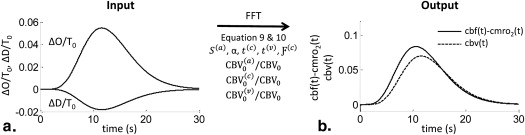
in which y ( t ) stands for either ΔO ( t ) or ΔD ( t ), t is time, and t 0 is the time at which brain activation starts. Γ represents the gamma function, which acts as a normalizing parameter, and δ and β are constants for which we set values of δ = 8 and β = 0.6 seconds −1 . The amplitude A was set to 3 μMs for ΔO ( t ) and −1 μMs for ΔD ( t ). These parameters were chosen to best represent typical hemodynamic signals during activation , as seen in Figure 1 a, where the ΔO ( t ) and ΔD ( t ) traces peak simultaneously at t − t 0 = 11.7s. We set the baseline total hemoglobin concentration T0 T
0 = 55 μM and the baseline tissue saturation S0 S
0 = 65%. These values fall within typical values reported in the literature for the human brain, which range between 42 and 79 μM for T0 T
0 , and between 55 and 75% for S0 S
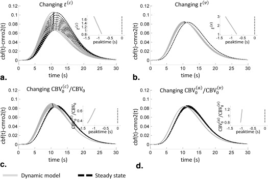
0 . Because the hemodynamic model depends on several parameters (as described previously), we have studied the sensitivity of cbf(t)−cmro2(t) cbf
(
t
)
−
cmro
2
(
t
) on the values assigned to these parameters. We further compared the model output with a steady-state approach that has been used extensively in the literature . In comparison to the dynamic model , a steady-state model does not consider any temporal shifts between cbf( t )—or cmro 2 ( t )—and ΔO ( t ) or ΔD ( t ). Mayhew et al. expressed the venous contributions to the tissue concentrations of D and T ( D(v) D
(
v
) , T(v) T
(
v
) ) in terms of the measurable overall tissue concentrations of D and T as follows :
ΔD(v)D(v)∣∣0−ΔT(v)T(v)∣∣0=γrΔDD0−γtΔTT0=−(cbf(t)−cmro2(t)). Δ
D
(
v
)
D
(
v
)
|
0
−
Δ
T
(
v
)
T
(
v
)
|
0
=
γ
r
Δ
D
D
0
−
γ
t
Δ
T
T
0
=
−
(
cbf
(
t
)
−
cmro
2
(
t
)
)
.
in which γr γ
r and γt γ
t have been assumed to be constants within the range 0.2 to 5 and D ( v ) 0 and T ( v ) 0 are the baseline deoxy hemoglobin concentration and total hemoglobin concentration in the venous compartment, respectively. Equation (26) fits in the definition of steady-state models because it introduces no temporal shift between the changes in the D and T hemoglobin concentrations ( D ( v ) , T ( v ) ), and the blood flow and oxygen consumption perturbations (cbf( t ), cmro 2 ( t )) that cause them. Recently, Fantini derived the following explicit expressions for the coefficients γr γ
r and γt γ
t , under the approximation (1−S(a))≅0 (
1
−
S
(
a
)
)
≅
0 :
γr=(1−<S(c)>)Ƒ(c)CBV(c)0CBV(v)0+(1−S(v))<S(c)>S(v)(<S(c)>−S(v))Ƒ(c)CBV(c)0CBV(v)0+(S(a)−S(v)), γ
r
=
(
1
−
<
S
(
c
)
)
Ƒ
(
c
)
CBV
0
(
c
)
CBV
0
(
v
)
+
(
1
−
S
(
v
)
)
<
S
(
c
)
S
(
v
)
(
<
S
(
c
)
−
S
(
v
)
)
Ƒ
(
c
)
CBV
0
(
c
)
CBV
0
(
v
)
+
(
S
(
a
)
−
S
(
v
)
)
,
γt=1−S(v)<S(c)>S(v)(<S(c)>−S(v))Ƒ(c)CBV(c)0CBV0+(S(a)−S(v))CBV(v)0CBV0ΔCBV(v)ΔCBV. γ
t
=
1
−
S
(
v
)
<
S
(
c
)
S
(
v
)
(
<
S
(
c
)
−
S
(
v
)
)
Ƒ
(
c
)
CBV
0
(
c
)
CBV
0
+
(
S
(
a
)
−
S
(
v
)
)
CBV
0
(
v
)
CBV
0
Δ
CBV
(
v
)
Δ
CBV
.
Get Radiology Tree app to read full this article<
Get Radiology Tree app to read full this article<
Frequency Domain
Get Radiology Tree app to read full this article<
Get Radiology Tree app to read full this article<
Table 1
Upper and Lower Limits for the Six Fitting Parameters of the Model
t ( c ) (s)t ( v ) (s)Ƒ(c)CBV(c)0CBV(v)0 Ƒ
(
c
)
CBV
0
(
c
)
CBV
0
(
v
) (CBV(a)0cbv(a))(CBV(v)0cbv(v)) (
CBV
0
(
a
)
cbv
(
a
)
)
(
CBV
0
(
v
)
cbv
(
v
)
) ω(AutoReg)c2π(Hz) ω
c
(
AutoReg
)
2
π
(
Hz
) kCBV(v)0CBV0 k
CBV
0
(
v
)
CBV
0 Lower limit 0.4 1 0.8 0.2 0 0.4 Upper limit 1.4 3 2.4 5 0.15 1.6
( a ) , contributions from arterial compartments; ( c ) , contributions from capillary compartments; CBV, cerebral blood volume; cbv, relative change in CBV with respect to baseline; k , inverse of the modified Grubb exponent; t ( c ) , capillary blood transit time in seconds (s); t , time; ( v ) , contributions from venous compartments; ω c , cutoff frequency of autoregulation.
Get Radiology Tree app to read full this article<
Results
Time Domain Results for cbv(t) and cbf (t) − cmro 2 (t)
Get Radiology Tree app to read full this article<
S0=S(a)CBV(a)0+S(a)1−exp(−αt(c))αt(c)Ƒ(c)CBV(c)0+S(a)exp(−αt(c))CBV(v)0CBV0. S
0
=
S
(
a
)
CBV
0
(
a
)
+
S
(
a
)
1
−
exp
(
−
α
t
(
c
)
)
α
t
(
c
)
Ƒ
(
c
)
CBV
0
(
c
)
+
S
(
a
)
exp
(
−
α
t
(
c
)
)
CBV
0
(
v
)
CBV
0
.
Get Radiology Tree app to read full this article<
Get Radiology Tree app to read full this article<
Get Radiology Tree app to read full this article<
Get Radiology Tree app to read full this article<
Get Radiology Tree app to read full this article<
Get Radiology Tree app to read full this article<
Frequency Domain Results
Get Radiology Tree app to read full this article<
|  |
Get Radiology Tree app to read full this article<
Get Radiology Tree app to read full this article<
Table 2
Results of the Fitting Procedure for the Six Parameters of the Model, Reported in Terms of Their Mean Value and Standard Deviation
t ( c ) (s)t ( v ) (s)Ƒ(c)CBV(c)0CBV(v)0 Ƒ
(
c
)
CBV
0
(
c
)
CBV
0
(
v
) (CBV(a)0cbv(a))(CBV(v)0cbv(v)) (
CBV
0
(
a
)
cbv
(
a
)
)
(
CBV
0
(
v
)
cbv
(
v
)
) ω(AutoReg)c2π(Hz) ω
c
(
AutoReg
)
2
π
(
Hz
) kCBV(v)0CBV0 k
CBV
0
(
v
)
CBV
0 Mean ± SD 0.92 ± 0.18 1.29 ± 0.26 1.08 ± 0.27 2.95 ± 0.85 0.035 ± 0.002 0.59 ± 0.10
( a ) , contributions from arterial compartments; ( c ) , contributions from capillary compartments; CBV, cerebral blood volume; cbv, relative change in CBV with respect to baseline; k , inverse of the modified Grubb exponent; t ( c ) , capillary blood transit time in seconds (s); t , time; ( v ) , contributions from venous compartments; ω c , cutoff frequency of autoregulation.
Get Radiology Tree app to read full this article<
Get Radiology Tree app to read full this article<
Discussion
Get Radiology Tree app to read full this article<
Get Radiology Tree app to read full this article<
Get Radiology Tree app to read full this article<
Get Radiology Tree app to read full this article<
Get Radiology Tree app to read full this article<
Get Radiology Tree app to read full this article<
Conclusions
Get Radiology Tree app to read full this article<
Get Radiology Tree app to read full this article<
Get Radiology Tree app to read full this article<
Get Radiology Tree app to read full this article<
References
1. Ferrari M., Quaresima V.: A brief review on the history of human functional near-infrared spectroscopy (fNIRS) development and fields of application. Neuroimage 2012; 63: pp. 921-935.
2. Hillman E.M.: Optical brain imaging in vivo: techniques and applications from animal to man. J Biomed Opt 2007; 12: pp. 051402.
3. Leff D.R., Oriheula-Espina F., Elwell C.E., et. al.: Assessment of the cerebral cortex during motor task behaviours in adults: a systematic review of functional near infrared spectroscopy (fNIRS) studies. Neuroimage 2011; 54: pp. 2922-2936.
4. Buxton R.B.: Dynamic models of BOLD contrast. Neuroimage 2012; 62: pp. 953-961.
5. Fantini S.: Dynamic model for the tissue concentration and oxygen saturation of hemoglobin in relation to blood volume, flow velocity, and oxygen consumption: implications for functional neuroimaging and coherent hemodynamics spectroscopy (CHS). Neuroimage 2014; 85: pp. 202-221.
6. Reinhard M., Ewhrle-Wieland E., Grabiak D., et. al.: Oscillatory cerebral hemodynamics—the macro- vs. microvascular level. J Neurol Sci 2006; 250: pp. 103-109.
7. Cheng R., Shang Y., Hayes D., et. al.: Noninvasive optical evaluation of spontaneous low frequency oscillations in cerebral hemodynamics. Neuroimage 2012; 62: pp. 1445-1454.
8. Claassen J.A., Levine B.D., Zhang R.: Dynamic cerebral autoregulation during repeated squat-stand maneuvers. J Appl Physiol 2009; 106: pp. 153-160.
9. Aaslid R., Blaha M., Sviri G., et. al.: Asymmetric dynamic cerebral autoregulatory response to cyclic stimuli. Stroke 2007; 38: pp. 1465-1469.
10. Pierro M.L., Hallacoglu B., Sassaroli A., et. al.: Validation of a novel hemodynamic model for coherent hemodynamics spectroscopy (CHS) and functional brain studies with fNIRS and fMRI. Neuroimage 2014; 85: pp. 222-233.
11. Fantini S.: A new hemodynamic model shows that temporal perturbations of cerebral blood flow and metabolic rate of oxygen cannot be measured individually using functional near-infrared spectroscopy. Physiol Measure 2014; 35:
12. Chen J.L., Wei L., Acuff V., et. al.: Slightly altered permeability-surface area products imply some cerebral capillary recruitment during hypercapnia. Microvasc Res 1994; 48: pp. 190-211.
13. Gobel U., Klein B., Schrock H., et. al.: Lack of capillary recruitment in the brains of awake rats during hypercapnia. J Cereb Blood Flow Metab 1989; 9: pp. 491-499.
14. Kuschinsky W., Paulson O.B.: Capillary circulation in the brain. Cerebrovasc Brain Metab Rev 1992; 4: pp. 261-286.
15. Villringer A.: The intravascular susceptibility effect and the underlying physiology of fMRI. Neuroimage 2012; 62: pp. 995-999.
16. Villringer A., Them A., Lindauer U., et. al.: Capillary perfusion of the rat brain cortex. An in vivo confocal microscopy study. Circ Res 1994; 75: pp. 55-62.
17. Zoccoli G., Lucchi M.L., Andreoli E., et. al.: Brain capillary perfusion during sleep. J Cereb Blood Flow Metab 1996; 16: pp. 1312-1318.
18. Fantini S.: A haemodynamic model for the physiological interpretation of in vivo measurements of the concentration and oxygen saturation of haemoglobin. Phys Med Biol 2002; 47: pp. N249-N257.
19. Blaber A.P., Bondar R.L., Stein F., et. al.: Transfer function analysis of cerebral autoregulation dynamics in autonomic failure patients. Stroke 1997; 28: pp. 1686-1692.
20. Diehl R.R., Linden D., Lucke D., et. al.: Phase relationship between cerebral blood-flow velocity and blood-pressure—a clinical-test of autoregulation. Stroke 1995; 26: pp. 1801-1804.
21. Zhang R., Zuckerman J.H., Giller C.A., et. al.: Transfer function analysis of dynamic cerebral autoregulation in humans. Am J Physiol 1998; 274: pp. H233-H241.
22. Masamoto K., Kershaw J., Ureshi M., et. al.: Apparent diffusion time of oxygen from blood to tissue in rat cerebral cortex: implication for tissue oxygen dynamics during brain functions. J Appl Physiol 2007; 103: pp. 1352-1358.
23. Friston K.J., Josephs O., Rees G., et. al.: Nonlinear event-related responses in fMRI. Magnet Reson Med 1998; 39: pp. 41-52.
24. Glover G.H.: Deconvolution of impulse response in event-related BOLD fMRI. Neuroimage 1999; 9: pp. 416-429.
25. Goutte C., Nielsen F.A., Hansen L.K.: Modeling the haemodynamic response in fMRI using smooth FIR filters. IEEE Trans Med Imaging 2000; 19: pp. 1188-1201.
26. Lindquist M.A., Meng Loh J., Atlas L.Y., et. al.: Modeling the hemodynamic response function in fMRI: efficiency, bias and mis-modeling. Neuroimage 2009; 45: pp. S187-S198.
27. Lindquist M.A., Wager T.D.: Validity and power in hemodynamic response modeling: a comparison study and a new approach. Hum Brain Mapp 2007; 28: pp. 764-784.
28. Medvedev A.V., Kainerstorfer J.M., Borisov S.V., et. al.: Functional connectivity in the prefrontal cortex measured by near-infrared spectroscopy during ultrarapid object recognition. J Biomed Opt 2011; 16: pp. 016008.
29. Sassaroli A., deB Frederick B., Tong Y., et. al.: Spatially weighted BOLD signal for comparison of functional magnetic resonance imaging and near-infrared imaging of the brain. Neuroimage 2006; 33: pp. 505-514.
30. Yucel M.A., Huppert T.J., Boas D.A., et. al.: Calibrating the BOLD signal during a motor task using an extended fusion model incorporating DOT, BOLD and ASL data. Neuroimage 2012; 61: pp. 1268-1276.
31. Hallacoglu B., Sassaroli A., Wysocki M., et. al.: Absolute measurement of cerebral optical coefficients, hemoglobin concentration and oxygen saturation in old and young adults with near-infrared spectroscopy. J Biomed Opt 2012; 17: pp. 081406-081411.
32. Gagnon L., Gauthier C., Hoge R.D., et. al.: Double-layer estimation of intra- and extracerebral hemoglobin concentration with a time-resolved system. J Biomed Opt 2008; 13: pp. 054019.
33. Ohmae E., Ouchi Y., Oda M., et. al.: Cerebral hemodynamics evaluation by near-infrared time-resolved spectroscopy: correlation with simultaneous positron emission tomography measurements. Neuroimage 2006; 29: pp. 697-705.
34. Gatto R., Hoffman W.E., Mueller M., et. al.: Age effects on brain oxygenation during hypercapnia. J Biomed Opt 2007; 12: pp. 062113.
35. Quaresima V., Ferrai M., Torricelli A., et. al.: Bilateral prefrontal cortex oxygenation responses to a verbal fluency task: a multichannel time-resolved near-infrared topography study. J Biomed Opt 2005; 10: pp. 11012.
36. Choi J., Wolf M., Toronov V., et. al.: Noninvasive determination of the optical properties of adult brain: near-infrared spectroscopy approach. J Biomed Opt 2004; 9: pp. 221-229.
37. Mayhew J., Johnston D., Berwick J., et. al.: Spectroscopic analysis of neural activity in brain: increased oxygen consumption following activation of barrel cortex. Neuroimage 2000; 12: pp. 664-675.
38. Mayhew J., Johnston D., Martindale J., et. al.: Increased oxygen consumption following activation of brain: theoretical footnotes using spectroscopic data from barrel cortex. Neuroimage 2001; 13: pp. 975-987.
39. Dunn A.K., Devor A., Dale A.M., et. al.: Spatial extent of oxygen metabolism and hemodynamic changes during functional activation of the rat somatosensory cortex. Neuroimage 2005; 27: pp. 279-290.
40. Roche-Labarbe N., Fenoglio A., Radhakrishnan H., et. al.: Somatosensory evoked changes in cerebral oxygen consumption measured non-invasively in premature neonates. Neuroimage 2014; 85: pp. 279-286.
41. Mayhew J., Johnston D., Berwick J., et. al.: Erratum and addendum. Spectroscopic analysis of neural activity in the brain: increased oxygen consumption following activation of barrel cortex. Neuroimage 2001; 13: pp. 540-543.
42. Jones M., Berwick J., Johnston D., et. al.: Concurrent optical imaging spectroscopy and laser-Doppler flowmetry: the relationship between blood flow, oxygenation, and volume in rodent barrel cortex. Neuroimage 2001; 13: pp. 1002-1015.
43. Pries A.R., Secomb T.W.: Blood flow in microvascular networks.Tuma R.F.Durán W.N.Ley K.Handbook of physiology: microcirculation.2008.Academic PressSan Diego:
44. Cassot F., Lauwers F., Fouard C., et. al.: A novel three-dimensional computer-assisted method for a quantitative study of microvascular networks of the human cerebral cortex. Microcirculation 2006; 13: pp. 1-18.
45. Grubb R.L., Raichle M.E., Eichling J.O., et. al.: The effects of changes in PaCO2 on cerebral blood volume, blood flow, and vascular mean transit time. Stroke 1974; 5: pp. 630-639.
46. Kida I., Rothman D.L., Hyder F.: Dynamics of changes in blood flow, volume, and oxygenation: implications for dynamic functional magnetic resonance imaging calibration. J Cereb Blood Flow Metab 2007; 27: pp. 690-696.
47. Leung T.S., Tachtsidis I., Tisdall M.M., et. al.: Estimating a modified Grubb’s exponent in healthy human brains with near infrared spectroscopy and transcranial Doppler. Physiol Measur 2009; 30: pp. 1-12.
48. Mandeville J.B., Marota J.J., Avata C., et. al.: MRI measurement of the temporal evolution of relative CMRO(2) during rat forepaw stimulation. Magn Reson Med 1999; 42: pp. 944-951.
49. Baumgärtl H., Lübbers D.W.: Microaxial needle sensor for polarographic measurement of local O2 pressure in the cellular range of living tissue: Its construction and properties.Gnaiger E.Forstner H.Polarographic oxygen sensors, aquatic and physiological applications.1983.Springer VerlagBerlin, Heidelberg, New York:
50. Kasischke K.A., Lambert E.M., Panepento B., et. al.: Two-photon NADH imaging exposes boundaries of oxygen diffusion in cortical vascular supply regions. J Cereb Blood Flow Metab 2011; 31: pp. 68-81.
51. Pardridge W.M.: Drug transport in brain via the cerebrospinal fluid. Fluids Barriers CNS 2011; 8: pp. 7.
52. Mintun M.A., Lundstrom B.N., Snyder A.Z., et. al.: Blood flow and oxygen delivery to human brain during functional activity: theoretical modeling and experimental data. Proc Natl Acad Sci U S A 2001; 98: pp. 6859-6864.
53. Masamoto K., Kurachi T., Takizawa N., et. al.: Successive depth variations in microvascular distribution of rat somatosensory cortex. Brain Res 2004; 995: pp. 66-75.
54. Gommer E.D., Shijaku E., Mess W.H., et. al.: Dynamic cerebral autoregulation: different signal processing methods without influence on results and reproducibility. Med Biol Engineering Comp 2010; 48: pp. 1243-1250.
55. Pierro M.L., Kainerstorfer J.M., Civiletto A., et. al.: Reduced speed of microvascular blood flow in hemodialysis patients versus healthy controls: a coherent hemodynamics spectroscopy study. J Biomed Opt 2013;