Prediction Accuracy of a Sample-size Estimation Method for ROC Studies

Rationale and Objectives

Sample-size estimation is an important consideration when planning a receiver operating characteristic (ROC) study. The aim of this work was to assess the prediction accuracy of a sample-size estimation method using the Monte Carlo simulation method.

Materials and Methods

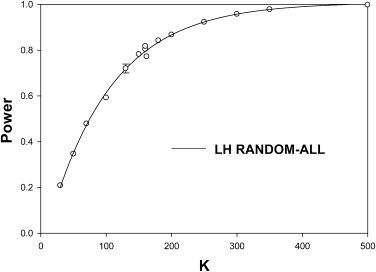
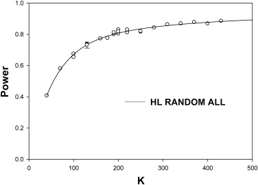
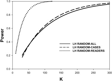
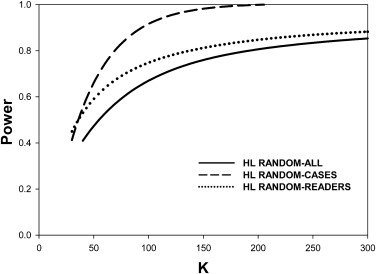
Two ROC ratings simulators characterized by low reader and high case variabilities (LH) and high reader and low case variabilities (HL) were used to generate pilot data sets in two modalities. Dorfman-Berbaum-Metz multiple-reader multiple-case (DBM-MRMC) analysis of the ratings yielded estimates of the modality-reader, modality-case, and error variances. These were input to the Hillis-Berbaum (HB) sample-size estimation method, which predicted the number of cases needed to achieve 80% power for 10 readers and an effect size of 0.06 in the pivotal study. Predictions that generalized to readers and cases (random-all), to cases only (random-cases), and to readers only (random-readers) were generated. A prediction-accuracy index defined as the probability that any single prediction yields true power in the 75%–90% range was used to assess the HB method.

Results

For random-case generalization, the HB-method prediction-accuracy was reasonable, ∼ 50% for five readers and 100 cases in the pilot study. Prediction-accuracy was generally higher under LH conditions than under HL conditions. Under ideal conditions (many readers in the pilot study) the DBM-MRMC–based HB method overestimated the number of cases. The overestimates could be explained by the larger modality-reader variance estimates when reader variability was large (HL). The largest benefit of increasing the number of readers in the pilot study was realized for LH, where 15 readers were enough to yield prediction accuracy >50% under all generalization conditions, but the benefit was lesser for HL where prediction accuracy was ∼36% for 15 readers under random-all and random-reader conditions.

Conclusion

The HB method tends to overestimate the number of cases. Random-case generalization had reasonable prediction accuracy. Provided about 15 readers were used in the pilot study the method performed reasonably under all conditions for LH. When reader variability was large, the prediction-accuracy for random-all and random-reader generalizations was compromised. Study designers may wish to compare the HB predictions to those of other methods and to sample-sizes used in previous similar studies.

The purpose of most imaging system assessment studies is to determine for a given diagnostic task whether radiologists perform better on one imaging system than another and whether the difference is statistically significant. In the receiver-operating characteristic (ROC) observer performance paradigm in which the radiologist assigns a rating to each patient image (ie, confidence level that the patient has disease), the performance index is usually chosen to be the area under the ROC curve (AUC ≡ A). The statistical analysis determines the significance level of the study (ie, the P value for rejecting the null hypothesis [NH] that the difference between the two AUCs is zero [ ΔA=0 Δ

0 ]). If the P value is smaller than a prespecified value α, typically set at 5%, one rejects the NH and declares the modalities different at the α significance level. Statistical power is the probability of rejecting the NH when the alternative hypothesis (AH) ΔA≠0 Δ

≠

0 is true. The difference ΔA Δ

A under the AH is referred to as the effect size.

Statistical power depends on the numbers of readers and cases, the variability of reader skill levels, the variability of difficulty levels of the cases, the statistical analysis used to estimate the P value, the effect size, and α. The aim of sample-size estimation methodology is to estimate the numbers of readers and cases needed to achieve the desired power for a specified analysis method, ΔA Δ

A , and α. Sample-size estimation is an important consideration at the planning stage of a study. An underpowered study (too few readers or cases) raise ethical issues because study patients are subjected to unnecessary imaging procedures for a study of questionable statistical strength. Conversely, an excessively overpowered study subjects unnecessarily large numbers of patients to imaging procedures and raises the cost of the study. It is generally considered preferable to err on the conservative side (ie, overpowered studies are preferred to underpowered studies), provided excessive overpowering is avoided. Studies are typically designed for 80% desired power.

Get Radiology Tree app to read full this article<

Methods

Overview of the Validation Methodology

Get Radiology Tree app to read full this article<

DBM-MRMC Analysis

Get Radiology Tree app to read full this article<

ijk=KAij−(K−1)Aij(k) i

−

(

−

)

(

)

In Equation 1 , ijk i

k is the pseudovalue corresponding to modality i (i = 1, 2, …, I), reader j (j = 1, 2, …, J), and case k (k = 1, 2, …, K), where I is the number of modalities (2 in this study), J is the number of readers, and K is the number of cases. Aij A

j is AUC for modality i and reader j when all cases are included in the analysis. Aij(k) A

(

) is AUC for modality i and reader j when case k is excluded from the analysis. The jackknife procedure is repeated for all modalities, readers, and cases, yielding a three-dimensional matrix containing IJK pseudovalues. In recent extensions to the original DBM-MRMC method by Hillis and Berbaum , the transformation ∗ijk=ijk+Aij−ij.¯¯¯. i

∗

−

. is applied to the pseudovalues (the bar denotes the average over the dotted index) and ∗ijk i

∗ is referred to as a normalized pseudovalue. In this work, normalized pseudovalues were used and the asterisk symbol is suppressed. Other changes from the original algorithm that are described elsewhere were also implemented.

Get Radiology Tree app to read full this article<

ijk=+τi+Rj+Ck+(τR)ik+(τC)ik+(RC)jk+εijk. i

(

)

(

)

(

)

The notation x∼N(0,σ2) x

∼

(

) denotes that x is a sample from a normal distribution with zero mean and variance σ2 σ

2 . According to Equation 2 each pseudovalue ijk i

k is assumed to be the sum of eight terms: a constant term representing the average over all modalities, readers and cases, estimated by …¯¯¯¯¯ …

¯ ; a modality effect τi τ

i estimated by i..¯¯¯ i

¯ ; a random contribution Rj∼N(0,σ2R) R

∼

(

) from the j th reader; a random contribution Ck∼N(0,σ2C) C

∼

(

) from the k th case; and second-order interaction contributions, modality-reader (τR)ij∼N(0,σ2τR) (

)

∼

(

) , which accounts for modality dependence of a reader’s contribution; modality-case (τC)ik∼N(0,σ2τC) (

)

∼

(

) ; reader-case (RC)jk∼N(0,σ2RC) (

)

∼

(

) , and an error term εijk∼N(0,σ2ε) ε

∼

(

) . For normalized pseudovalues, it can be shown that for two modalities |2..¯¯¯−1..¯¯¯|=ΔAˆ |

−

ˆ , an estimate of the effect size. The estimate is subject to sampling variability, but when averaged over many simulations, the estimated effect size approaches the ratings-simulator (see the following section) specified effect size ΔA=0.06 Δ

0.06 . The variances σ2R σ

2 , σ2C σ

2 , σ2τR σ

2 , σ2τC σ

2 , σ2RC σ

2 , and σ2ε σ

2 are referred to as variance components. DBM-MRMC software analyzes the pseudovalue matrix using a customized mixed model analysis of variance procedure . The procedure yields the P value for rejecting the NH: τ1=τ2 τ

2 and estimates of the variance components.

Get Radiology Tree app to read full this article<

HB Sample-size Estimation Method

Get Radiology Tree app to read full this article<

Roe and Metz Decision Variable Simulator

Get Radiology Tree app to read full this article<

Table 1

Z-sample and the Pseudovalue Variance Components for the Two Simulators used in this Work

z-sample Variance Components Simulator(σZR)2 (

)

2 (σZC)2 (

)

2 (σZRC)2 (

)

2 (σZτR)2 (

)

2 (σZτC)2 (

)

2 (σZϵ)2 (

)

2 LH 0.0055 0.3 0.2 0.0055 0.3 0.2 HL 0.0300 0.1 0.2 0.0300 0.1 0.6 Pseudovalue variance components Simulatorσ2R σ

2 σ2C σ

2 σ2RC σ

2 σ2τR σ

2 σ2τC σ

2 σ2ϵ σ

2 LH 2.82E-4

(1.8E-1) 5.35E-2

(1.2E-2) 4.68E-2

(7.2E-3) 1.97E-4

(2.7E-1) 3.90E-2

(1.3E-2) 4.17E-2

(2.5E-3) HL 1.69E-3

(5.3E-2) 1.54E-2

(1.4E-2) 7.24E-2

(6.9E-3) 4.77E-4

(6.4E-2) 1.06E-2

(2.0E-2) 9.68E-2

(3.2E-3)

The pseudovalue variance components represent grand averages of multiple (at least 5) independent medians obtained from DBM-MRMC analysis of 2000 pilot data sets, each with 5 readers and 100 cases. The coefficients of variance (CVs) of the medians are listed in parentheses. Only the last three pseudovalue variance components are relevant to sample-size estimation. The CV of σ2τR σ

2 was larger than that of σ2τC σ

2 or σ2ϵ σ

2 . The variance of σ2τR σ

2 was about 2.4 times as large for HL than for LH.

Get Radiology Tree app to read full this article<

Determination of True Power

Get Radiology Tree app to read full this article<

Validation of the HB Method

Get Radiology Tree app to read full this article<

Results

Get Radiology Tree app to read full this article<

Table 2

Summary of the Predictions of the HB Method Using Simulated Pilot Datasets with 5 readers, 50 Normal and 50 Abnormal Cases and Effect-Size 0.06

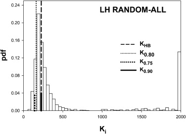
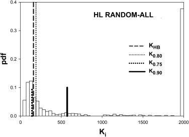
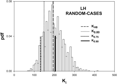
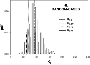
Simulator GeneralizationK0.80 K

0.80 KHB K

B PHB P

B fmax f

max Q0.75,0.90 Q

0.75

0.90 LH All 162 225 0.899 0.133 0.377 Cases 149 194 0.886 0.000 0.528 Readers 41 47 0.845 0.046 0.447 HL All 190 159 0.772 0.389 0.260 Cases 69 92 0.891 0.000 0.480 Readers 138 80 0.704 0.383 0.208

HB, Hillis-Berbaum; HL, high reader variability and low case variability; LH, low reader variability and high case variability.

Listed are the number of cases K0.80 K

0.80 for 80% true power; the median HB-predicted number of cases KHB K

B ; the corresponding true power PHB P

B ; the clipping fraction fmax f

max for KMAX=2000 K

MAX

2000 and the prediction-accuracy Q0.75,0.90 Q

0.75

0.90 . Prediction-accuracy was higher for LH. Prediction-accuracy was lower for HL, except for random cases, for which reader variability is set to zero. On the whole the HB method overestimates the number of cases. The two underestimates under HL changed to overestimates when the number of readers was increased sufficiently (see Table 3 ).

Get Radiology Tree app to read full this article<

Table 3

Effect of Increasing the Numbers of Readers in the Pilot Study

Simulator GeneralizationRPIL R

L KHB K

B PHB P

B fmax f

max Q0.75,0.90 Q

0.75

0.90 LH All 5 225 0.899 0.133 0.377 10 219 0.892 0.049 0.436 15 219 0.892 0.019 0.483 20 217 0.889 0.005 0.520 30 219 0.892 0.001 0.509 Readers 5 47 0.845 0.046 0.447 10 51 0.870 0.011 0.540 15 51 0.870 0.002 0.573 20 51 0.870 0.001 0.592 30 53 0.881 0.000 0.620 HL All 5 159 0.772 0.389 0.260 10 194 0.803 0.395 0.320 15 204 0.810 0.403 0.355 20 219 0.819 0.418 0.379 30 283 0.847 0.367 0.455 Readers 5 80 0.704 0.383 0.208 10 118 0.776 0.392 0.303 15 147 0.809 0.389 0.361 20 160 0.821 0.390 0.342 30 174 0.831 0.410 0.387

HB, Hillis-Berbaum; HL, high reader variability and low case variability; LH, low reader variability and high case variability; R PIL , number of readers in pilot study.

The prediction-accuracy Q0.70,0.95 Q

0.70

0.95 increased as RPIL R

L increased implying more pilot study readers are always helpful. The largest benefits were realized for LH, where 15 readers were enough to yield prediction accuracy >50% under all generalization conditions, but the benefits were lesser for HL. For the same RPIL R

L and generalization scenario Q0.70,0.90 Q

0.70

0.90 was larger for LH than for HL. Under ideal condition of many readers in the pilot study the HB-method was conservative under all conditions and prediction-accuracy approached 62%.

Get Radiology Tree app to read full this article<

Discussion

Get Radiology Tree app to read full this article<

Conclusions

Get Radiology Tree app to read full this article<

Acknowledgments

Get Radiology Tree app to read full this article<

Appendix A

Dataset Simulator for Random-readers and Cases

Get Radiology Tree app to read full this article<

Zijkt=μt+(Δμ)it+Rzjt+(Czkt)+(μR)zijk+(μC)zikt+(RC)zikt+(μRC)zikt Z

(

)

(

)

(

)

(

)

(

)

(

)

To simulate z-samples for random-cases, one sets (σzR)2=(σzτR)2=0 (

)

(

)

0 , which does not affect the normalization requirement (σzC)2+(σzτC)2+(σzRC)2+(σzε)2=1 (

)

(

)

(

)

(

)

1 . The simulation model was

zijkt=μt+(Δμ)it+Czkt+(τC)zikt+(RC)zjkt+εzijkt z

(

)

(

)

(

)

Get Radiology Tree app to read full this article<

(σza)2=(σzRC)2(σzRC)2+(σzε)2(σzb)2=(σzε)2(σzRC)2+(σzε)2 (

)

(

)

(

)

(

)

(

)

(

)

(

)

(

)

Note that (σza)2+(σzb)2=1 (

)

(

)

1 , ensuring that the simulator is properly normalized. The simulation model was

zijkt=μt+(Δμ)it+Rzjt+(τR)zijt+(RC)zjkt+εzijkt. z

(

)

(

)

(

)

where

(RC)jkt∼N(0,(σza)2)εijkt∼N(0,(σzb)2). (

)

∼

(

)

∼

(

)

Get Radiology Tree app to read full this article<

Appendix B

Hillis Berbaum Sample-size Estimation Formulae for Random-all

Get Radiology Tree app to read full this article<

nc=sqrt(RK)(ΔA)2/(Kσ2τR+Rσ2τC+σ2ε). n

(

)

(

)

(

)

Get Radiology Tree app to read full this article<

ddf=(R−1)((Kσ2τR+Rσ2τC+σ2ε)/(Kσ2τR+σ2ε))2. d

(

−

)

(

)

(

)

If σ2τC≤0 σ

≤

ddf=(R−1). d

(

−

)

Get Radiology Tree app to read full this article<

power≈prob(F1,ddf,nc>F1−α;1,ddf). p

≈

(

−

;

)

Get Radiology Tree app to read full this article<

References

1. Kundel H.L., Berbaum K.S., Dorfman D.D., et. al.: Receiver Operating Characteristic Analysis in Medical Imaging. ICRU Report 79 2008; 8
2. Lenth R.V.: Some practical guidelines for effective sample size determination. Am Stat 2001; 55: pp. 187-193.
3. Obuchowski N.A.: How many observers are needed in clinical studies of medical imaging?. Am J Roentgenol 2004; 182: pp. 867-869.
4. Obuchowski N.: Determining sample size for roc studies: what is reasonable for the expected difference in tests in ROC areas?. Acad Radiol 2003; 10: pp. 1327-1328.
5. Hanley J.A., McNeil B.J.: A method of comparing the areas under receiver operating characteristic curves derived from the same cases. Radiology 1983; 48: pp. 839-843.
6. Obuchowski N.A.: Computing sample size for receiver operating characteristic studies. Invest Radiol 1994; 29: pp. 238-243.
7. Obuchowski N.A., McLish D.K.: Sample size determination for diagnostic accuracy studies involving binormal ROC curve indices. Stat Med 1997; 16: pp. 1529-1542.
8. Metz C.E.: ROC methodology in radiologic imaging. Investi Radiol 1986; 21: pp. 720-733.
9. Obuchowski N.A.: Multireader, multimodality receiver operating characteristic curve studies: hypothesis testing and sample size estimation using an analysis of variance approach with dependent observations. Acad Radiol 1995; 2: pp. S22-S29.
10. Hillis S.L., Berbaum K.S.: Power estimation for the Dorfman-Berbaum-Metz method. Acad Radiol 2004; 11: pp. 1260-1273.
11. Beiden S.V., Wagner R.F., Campbell G.: Components of variance models and multiple-bootstrap experiments: an alternative method for random-effects, receiver operating characteristic analysis. Acad Radiol 2000; 7: pp. 341-349.
12. Obuchowski N.A.: Sample size calculations in studies of test accuracy. Stat Methods Med Res 1998; 7: pp. 371-392.
13. Obuchowski N.A.: Sample size tables for receiver operating characteristic studies. Am J Roentgenol 2000; 175: pp. 603-608.
14. Zhou X.-H., Obuchowski N.A., McClish D.K.: Statistical methods in diagnostic medicine.2002.John Wiley & SonsNew York
15. Pepe M.S.: The statistical evaluation of medical tests for classification and prediction. Oxford Statistical Science Series.2003.Oxford University PressNew York
16. Obuchowski N.: Reducing the number of reader interpretations in MRMC studies. Acad Radiol 2009; 16: pp. 209-217.
17. Roe C.A., Metz C.E.: Dorfman-Berbaum-Metz method for statistical analysis of multireader, multimodality receiver operating characteristic data: validation with computer simulation. Acad Radiol 1997; 4: pp. 298-303.
18. Dorfman DD, Berbaum KS, Lenth RV, et al. Monte Carlo validation of a multireader method for receiver operating characteristic discrete rating data: split-plot experimental design. Medical Imaging 1999: Image Perception and Performance, 1999, San Diego, CA.
19. Obuchowski N.A., Rockette H.E.: Hypothesis testing of the diagnostic accuracy for multiple diagnostic tests: an ANOVA approach with dependent observations. Commun Stat Simulat Comp 1995; 24: pp. 285-308.
20. Hillis S.L., Berbaum K.S.: Monte Carlo validation of the Dorfman-Berbaum-Metz method using normalized pseudovalues and less data-based model simplification. Acad Radiol 2005; 12: pp. 1534-1541.
21. Dorfman D.D., Berbaum K.S., Lenth R.V., et. al.: Monte Carlo validation of a multireader method for receiver operating characteristic discrete rating data: factorial experimental design. Acad Radiol 1998; 5: pp. 591-602.
22. Matsumoto M., Nishimura T.: Mersenne twister—a 623-dimensionally equidistributed uniform pseudorandom number generator. ACM Trans Modeling Comp Simulation 1998; 8: pp. 3-30.
23. Galassi M., Davies J., Theiler J., et. al.: GNU Scientific Library Reference Manual. 1.6.2005.Network Theory LimitedBristol, UK
24. Dorfman D.D., Berbaum K.S., Metz C.E.: ROC characteristic rating analysis: generalization to the population of readers and patients with the jackknife method. Invest Radiol 1992; 27: pp. 723-731.
25. Hillis S.L., Berbaum K.S., Metz C.E.: Recent developments in the Dorfman-Berbaum-Metz procedure for multireader ROC study analysis. Acad Radiol 2008; 15: pp. 647-661.
26. Roe C.A., Metz C.E.: Variance-component modeling in the analysis of receiver operating characteristic index estimates. Acad Radiol 1997; 4: pp. 587-600.
27. Hillis SL, Berbaum KS. MRMC sample size program user guide. Available from http://perception.radiology.uiowa.edu . Accessed December 28, 2009.
28. Berbaum KS, Metz CE, Pesce LL, et al. DBM MRMC user’s guide, DBM-MRMC 2.1 Beta Version 2. Available from http://www-radiology.uchicago.edu/cgi-bin/roc_software.cgi and from http://perception.radiology.uiowa.edu . Accessed December 28, 2009.
29. Burgess A.E.: Comparison of receiver operating characteristic and forced choice observer performance measurement methods. Med Phys 1995; 22: pp. 643-655.
30. Kreaemer H.C., Mintz J., Noda A., et. al.: Caution regarding the use of pilot studies to guide power calculations for study proposals. Arch Gen Psychiatry 2006; 63: pp. 484-489.

Prediction Accuracy of a Sample-size Estimation Method for ROC Studies

Rationale and Objectives

Materials and Methods

Results

Conclusion

Methods

Overview of the Validation Methodology

DBM-MRMC Analysis

HB Sample-size Estimation Method

Roe and Metz Decision Variable Simulator

Determination of True Power

Validation of the HB Method

Results

Discussion

Conclusions

Acknowledgments

Appendix A

Dataset Simulator for Random-readers and Cases

Appendix B

Hillis Berbaum Sample-size Estimation Formulae for Random-all

References

Further Reading

Antiangiogenic Tumor Treatment

CT Guided Percutaneous Cryoneurolysis for Post Thoracotomy Pain Syndrome

Decision Analytic Model for Evaluation of Suspected Coronary Disease with Stress Testing and Coronary CT Angiography