Prediction of Perceptible Artifacts in JPEG2000 Compressed Abdomen CT Images Using a Perceptual Image Quality Metric

Rationale and Objectives

To test a perceptual quality metric (high-dynamic range visual difference predictor, HDR-VDP) in predicting perceptible artifacts in Joint Photographic Experts Group 2000 compressed thin- and thick-section abdomen computed tomography images.

Materials and Methods

A total of 120 thin (0.67 mm) and corresponding thick (5 mm) sections were compressed to ratios from 4:1 to 15:1. Peak signal-to-noise ratio (PSNR), HDR-VDP results (paired t -tests), and five radiologists’ pooled responses for the presence of artifacts (exact tests for paired proportions) were compared between the thin and thick sections. For three subsets of 120 thin- (subset A), 120 thick- (subset B), and 60 thin- and 60 thick-section compressed images (subset C), receiver operating curve analysis was performed to compare PSNR and HDR-VDP in predicting the radiologists’ responses. Using the cutoff values where the sum of sensitivity and specificity was the maximum in subset C, visually lossless thresholds (VLTs) were estimated for the 240 original images and the estimation accuracy was compared (McNemar test).

Results

Thin sections showed more artifacts in terms of PSNR, HDR-VDP, and radiologists’ responses ( p < .0001). HDR-VDP outperformed PSNR for subset C (area under the curve: 0.97 versus 0.93, p = 0.03), whereas they did not differ significantly for subset A or B. Using the cutoff values, PSNR and HDR-VDP predicted the VLT accurately for 124 (51.7%) and 183 (76.3%) images, respectively ( p < .0001).

Conclusions

HDR-VDP can predict the perceptible compression artifacts, and therefore can be potentially used to estimate the VLT for such compressions.

Irreversible image compression appears to be an immediate and effective means to reduce enormous data ( ) generated by modern computed tomography (CT) scanners ( ). Previous studies ( ) have reported acceptable compression levels for CT images as 8:1 to 20:1. Most of these investigated a compression threshold that does not cause a loss of diagnostic information. However, it is difficult to generalize such study results, because the diagnostically lossless threshold varies with diagnostic tasks ( ). For instance, it has been reported that detection performance of CT for hepatic nodules is preserved with up to 10:1 compression ( ); however, it is uncertain whether this compression level is acceptable for the characterization of the nodules and for the detection of any coincidental findings which might be clinically important in the same CT dataset. Furthermore, compression artifacts are affected by image content itself ( ) and scanning parameters such as section thickness ( ). Therefore it is very unlikely that a reported acceptable compression level for images of a certain type (eg, abdomen CT) can be an optimal compression guideline for all images of the same type.

If a compressed image is indistinguishable from its original, there is no basis for arguing the compression hinders any diagnostic accuracy ( ). Although this visually lossless threshold (VLT) allows relatively low-level compressions, it has been gaining support as a practicable compression level ( ). To estimate the VLT, human readers need to determine whether a compressed image is distinguishable from its original or not at various compression levels, which seems impractical in clinical practice.

Get Radiology Tree app to read full this article<

Materials and methods

Get Radiology Tree app to read full this article<

CT Scanning

Get Radiology Tree app to read full this article<

Table 1

Lesions in 120 Original Thick Sections

Lesion Number of Images Normal 70 Cystic focal lesion in the solid organ 6 Arterial luminal irregularity or wall calcification 5 Peritoneal carcinomatosis or peritonitis 5 Tube, anastomosis, or other postoperative finding 5 Bowel wall thickening 4 Solid focal lesion in the solid organ 4 Acute appendicitis 3 Ascites or pleural effusion 3 Acute pancreatitis or retroperitoneal edema 2 Colonic diverticulosis or diverticulitis 2 Focal calcification or stone 2 Gall bladder distension or wall thickening 2 Lymph node enlargement 2 Organ enlargement or atrophy 2 Severe bowel distension 2 Biliary dilatation 1

Get Radiology Tree app to read full this article<

Image Compression

Get Radiology Tree app to read full this article<

Table 2

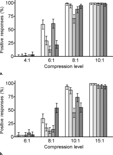
Actual Compression Levels, PSNR and HDR-VDP Results, and Pooled Readers’ Responses

Nominal Compression Level Actual Compression Level ⁎ PSNR (dB) HDR-VDP Readers’ Responses † Thin Thick Thin Thick Thin Thick Thin Thick 4:1 4.0 ± 0.1 — 52.9 ± 2.4 — 2.8 ± 2.4 — 0% (0/120) — 6:1 6.0 ± 0.1 6.2 ± 0.4 46.3 ± 3.0 53.7 ± 1.7 21.0 ± 13.4 3.4 ± 2.1 35.0% (42/120) 0% (0/120) 8:1 8.0 ± 0.0 8.0 ± 0.0 42.3 ± 3.1 50.7 ± 2.5 50.6 ± 21.1 12.4 ± 7.5 95.0% (114/120) 21.7% (26/120) 10:1 10.0 ± 0.1 10.0 ± 0.1 39.7 ± 3.1 48.2 ± 2.5 82.5 ± 26.2 29.9 ± 13.9 100% (120/120) 81.7% (98/120) 15:1 — 15.0 ± 0.1 — 44.0 ± 2.5 — 79.1 ± 22.5 — 100% (120/120)

PSNR: peak signal-to-noise ratio; HDR-VDP: high-dynamic range visual difference predictor.

Data are mean ± standard deviations.

Get Radiology Tree app to read full this article<

Human Observer Analysis

Get Radiology Tree app to read full this article<

VLT

Get Radiology Tree app to read full this article<

Peak Signal-to-Noise Ratio

Get Radiology Tree app to read full this article<

PSNR=20log10(255RMSE), P

log

⁡

(

255

)

where

RMSE(root - mean - square error)=∑512x=1∑512y=1(f(x,y)−g(x,y))25122−−−−−−−−−−−−−−−−−√, R

(

root - mean - square error

)

∑

512

∑

512

(

)

−

(

)

512

where f(x, y) and g(x, y) are the pixel values in the original and compressed images, respectively.

Get Radiology Tree app to read full this article<

Perceptual Model

Get Radiology Tree app to read full this article<

Statistical Analysis

Get Radiology Tree app to read full this article<

Results

Get Radiology Tree app to read full this article<

Table 3

Results of ROC Analysis

PSNR HDR-VDP_P_ Value Subset A (120 thin sections) AUC 0.98 (0.94–0.99) 0.99 (0.95, 0.99) .35 Cutoff value yielding the maximum sum of sensitivity and specificity 45.6 dB 24.8 Sensitivity (%) 95.6 (87.6–99.0) 94.1 (85.6–98.3) Specificity (%) 92.3 (81.4–97.8) 100 (93.1–100) Cutoff value yielding 100% sensitivity 47.0 dB 14.8 Specificity (%) 76.9 (63.2–87.5) 80.8 (67.5–90.4) Subset B (120 thick sections) AUC 0.97 (0.93–0.99) 0.98 (0.93–0.99) .53 Cutoff value yielding the maximum sum of sensitivity and specificity 49.7 dB 18.0 Sensitivity (%) 90.2 (79.8–96.3) 91.8 (81.9–97.3) Specificity (%) 96.6 (88.3–99.5) 100 (93.9–100) Cutoff value yielding 100% sensitivity 52.3 dB 6.5 Specificity (%) 57.6 (44.1–70.4) 54.2 (40.8–67.3) Subset C (60 thin and 60 thick sections) AUC 0.93 (0.87–0.97) 0.97 (0.92–0.99) .03 Cutoff value yielding the maximum sum of sensitivity and specificity 48.4 dB 20.3 Sensitivity (%) 89.4 (79.4–95.6) 89.3 (79.4–95.6) Specificity (%) 83.3 (70.7–92.1) 100 (93.3–100) Cutoff value yielding 100% sensitivity 52.3 dB 6.5 Specificity (%) 53.7 (39.6–67.4) 59.3 (45.0–72.4)

PSNR: peak signal-to-noise ratio; HDR-VDP: high-dynamic range visual difference predictor; ROC: receiver operating characteristic; AUC: area under the curve.

Data in parentheses are the 95% confidence intervals.

Get Radiology Tree app to read full this article<

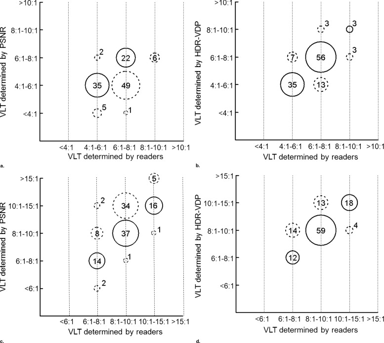
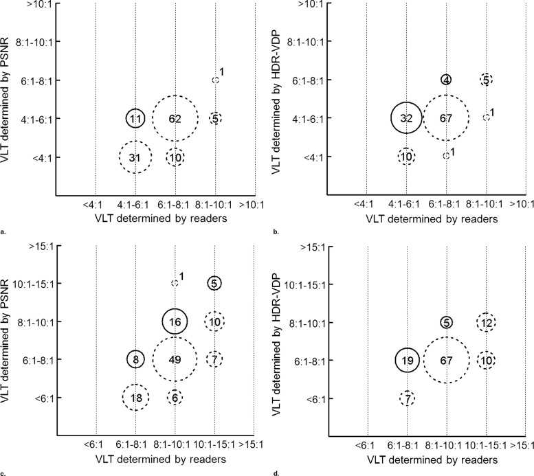
Table 4

VLT Range Prediction for 120 Thin and 120 Thick Sections Using the Cutoff Values Determined from ROC Analyses for Subset C

Concordant Underestimated Overestimated Cutoff value yielding the maximum sum of sensitivity and specificity PSNR 124 (57, 67) 65 (61, 4) 51 (2, 49) HDR-VDP 183 (94, 89) 20 (16, 4) 37 (10, 27) Cutoff value yielding 100% sensitivity PSNR 40 (11, 29) 199 (109, 90) 1 (0, 1) HDR-VDP 60 (36, 24) 180 (84, 96) 0 (0, 0)

See Table 3 for abbreviations.

Data are the number of images. Data in parentheses (separated by a comma) are the numbers of thin and thick sections.

Get Radiology Tree app to read full this article<

Discussion

Get Radiology Tree app to read full this article<

Acknowledgments

Get Radiology Tree app to read full this article<

References

1. Erickson B.J., Manduca A., Palisson P., et. al.: Wavelet compression of medical images. Radiology 1998; 206: pp. 599-607.
2. Schomer D.F., Elekes A.A., Hazle J.D., et. al.: Introduction to wavelet-based compression of medical images. Radiographics 1998; 18: pp. 469-481.
3. Bak P.R.G.: Will the use of irreversible compression become a standard of practice?. http://www.scarnet.org/pdf/SCARNews_Winter06.pdf Accessed July 28, 2006
4. Lee K.H., Lee H.J., Kim J.H., et. al.: Managing the CT data explosion: initial experiences of archiving volumetric datasets in a mini-PACS. J Digit Imaging 2005; 18: pp. 188-195.
5. Rubin G.D.: Data explosion: the challenge of multidetector-row CT. Eur J Radiol 2000; 36: pp. 74-80.
6. Tamm E.P., Thompson S., Venable S.L., McEnery K.: Impact of multislice CT on PACS resources. J Digit Imaging 2002; 15: pp. 96-101.
7. Cosman P.C., Davidson H.C., Bergin C.J., et. al.: Thoracic CT images: effect of lossy image compression on diagnostic accuracy. Radiology 1994; 190: pp. 517-524.
8. Goldberg M.A., Gazelle G.S., Boland G.W., et. al.: Focal hepatic lesions: effect of three-dimensional wavelet compression on detection at CT. Radiology 1997; 202: pp. 159-165.
9. Ko J.P., Chang J., Bomsztyk E., et. al.: Effect of CT image compression on computer-assisted lung nodule volume measurement. Radiology 2005; 237: pp. 83-88.
10. Ko J.P., Rusinek H., Naidich D.P., et. al.: Wavelet compression of low-dose chest CT data: effect on lung nodule detection. Radiology 2003; 228: pp. 70-75.
11. Li F., Sone S., Takashima S., et. al.: Effects of JPEG and wavelet compression of spiral low-dose CT images on detection of small lung cancers. Acta Radiol 2001; 42: pp. 156-160.
12. Megibow A.J., Rusinek H., Lisi V., et. al.: Computed tomography diagnosis utilizing compressed image data: an ROC analysis using acute appendicitis as a model. J Digit Imaging 2002; 15: pp. 84-90.
13. Ohgiya Y., Gokan T., Nobusawa H., et. al.: Acute cerebral infarction: effect of JPEG compression on detection at CT. Radiology 2003; 227: pp. 124-127.
14. Zalis M.E., Hahn P.F., Arellano R.S., et. al.: CT colonography with teleradiology: effect of lossy wavelet compression on polyp detection-initial observations. Radiology 2001; 220: pp. 387-392.
15. Zheng L.M., Sone S., Itani Y., et. al.: Effect of CT digital image compression on detection of coronary artery calcification. Acta Radiol 2000; 41: pp. 116-121.
16. Kim TJ, Lee KW, Kim B, et al. Regional variance of visually lossless threshold in compressed chest CT Images: lung versus mediastinum and chest Wall. Eur J Radiol. In press.
17. Woo H.S., Kim K.J., Kim T.J., et. al.: JPEG 2000 compression of abdominal CT: difference in compression tolerance between thin- and thick-section images. Am J Roentgenol 2007; 189: pp. 535-541.
18. Slone R.M., Foos D.H., Whiting B.R., et. al.: Assessment of visually lossless irreversible image compression: comparison of three methods by using an image-comparison workstation. Radiology 2000; 215: pp. 543-553.
19. Ringl H., Schernthaner R.E., Bankier A.A., et. al.: JPEG2000 compression of thin-section CT images of the lung: effect of compression ratio on image quality. Radiology 2006; 240: pp. 869-877.
20. Slone R.M., Muka E., Pilgram T.K.: Irreversible JPEG compression of digital chest radiographs for primary interpretation: assessment of visually lossless threshold. Radiology 2003; 228: pp. 425-429.
21. Lee K.H., Kim Y.H., Kim B.H., et. al.: Irreversible JPEG 2000 compression of abdominal CT for primary interpretation: assessment of visually lossless threshold. Eur Radiol 2007; 17: pp. 1529-1534.
22. Kim B, Lee KH, Kim KJ, et al. Prediction of perceptible artifacts in JPEG2000 compressed chest CT images using mathematical and perceptual quality metrics. Am J Roentgenol. In press.
23. Krupinski E.A., Kallergi M.: Choosing a radiology workstation: technical and clinical considerations. Radiology 2007; 242: pp. 671-682.
24. Mantiuk R., Daly S., Myszkowski K., et. al.: Predicting visible differences in high dynamic range images-model and its calibration. Proc Human Vision and Electronic Imaging X, IS&T/SPIE’s 17th Annual Symposium on Electronic Imaging 2005; pp. 204-214.
25. Mahesh M., Scatarige J.C., Cooper J., et. al.: Dose and pitch relationship for a particular multislice CT scanner. Am J Roentgenol 2001; 177: pp. 1273-1275.
26. Kim KJ, Kim B, Choi SW, et al. Definition of compression ratio: difference between two commercial JPEG2000 program libraries. Telemed J E Health. In press.
27. Digital Imaging and Communications in Medicine (DICOM). Part 14: gray scale standard display function. NEMA standards publication no. PS 3.14-2006.2006.National Electrical Manufacturers AssociationVa
28. Wang Z., Sheikh H.R., Bovik A.C.: Objective video quality assessment.Furht B.Marqure O.The handbook of video databases: design and applications.2003.CRC PressBoca Raton, FL:pp. 1041-1078.
29. Quick R.F.: A vector magnitude model of contrast detection. Kybernetik 1974; 16: pp. 65-67.
30. Eckert M.P., Bradley A.P.: Perceptual quality metrics applied to still image compression. Signal Processing 1998; 70: pp. 177-200.
31. Fleiss J.L., Cuzick J.: The reliability of dichotomous judgements: unequal numbers of judges per subject. Appl Psychol Measurement 1979; 3: pp. 537-542.
32. Persons K., Palisson P., Manduca A., et. al.: An analytical look at the effects of compression on medical images. J Digit Imaging 1997; 10: pp. 60-66.
33. Daly S.: The visible differences predictor: an algorithm for the assessment of image fidelity.Watson A.B.Digital images and human vision.1993.MIT PressCambridge, MA:pp. 179-206.
34. Lubin J.: The use of psychophysical data and models in the analysis of display system performance.Watson A.B.Digital images and human vision.1993.MIT PressCambridge, MA:pp. 163-178.
35. Siddiqui K.M., Siegel E.L., Reiner B.I., et. al.: Correlation of radiologists’ image quality perception with quantitative assessment parameters: just-noticeable difference vs. peak signal-to-noise ratios. Proc SPIE 2005; 5748: pp. 58-64.
36. Krupinski E.A., Johnson J., Roehrig H., et. al.: Using a human visual system model to optimize soft-copy mammography display. Acad Radiol 2003; 10: pp. 1030-1035.
37. Li B., Meyer G.W., Klassen R.V.: A comparison of two image quality models. Proc SPIE 1998; 3299: pp. 98-109.
38. Lubin J., Brill M.H., Crane R.L.: Vision model-based assessment of distortion magnitudes in digital video. http://www.mpeg.org/MPEG/JND/ Accessed July 4, 2006
39. Daly S.: A visual model for optimizing the design of image processing algorithms. IEEE Int Conf Image Proc 1994; pp. 16-20.
40. Siddiqui K.M., Johnson J.P., Reiner B.I., et. al.: Discrete cosine transform JPEG compression vs. 2D JPEG2000 compression: JNDmetrix visual discrimination model image quality analysis. Proc SPIE 2005; 5748: pp. 202-207.
41. Mantiuk R.: HDR visual difference predictor. http://sourceforge.net/projects/hdrvdp Accessed July 4, 2006
42. Eskicioglu A.M., Fisher P.S.: Image quality measures and their performance. IEEE Trans Comm 1995; 43: pp. 2959-2965.
43. Final report from the video quality experts group on the validation of objective models of video quality assessment, phase II. http://www.its.bldrdoc.gov/vqeg/projects/frtv_phaseII/downloads/VQEGII_Final_Report.pdf Accessed July 4, 2006
44. Wang Z., Bovik A.C., Sheikh H.R., et. al.: Image quality assessment: from error visibility to structural similarity. IEEE Trans Image Proc 2004; 13: pp. 600-612.
45. Lee K.H., Kim Y.H., Hahn S., et. al.: Computed tomography diagnosis of acute appendicitis: advantages of reviewing thin-section datasets using sliding slab average intensity projection technique. Invest Radiol 2006; 41: pp. 579-585.
46. Prokop M.: Multislice CT: technical principles and future trends. Eur Radiol 2003; 13: pp. M3-M13.

Prediction of Perceptible Artifacts in JPEG2000 Compressed Abdomen CT Images Using a Perceptual Image Quality Metric

Rationale and Objectives

Materials and Methods

Results

Conclusions

Materials and methods

CT Scanning

Image Compression

Human Observer Analysis

VLT

Peak Signal-to-Noise Ratio

Perceptual Model

Statistical Analysis

Results

Discussion

Acknowledgments

References

Further Reading

30% unnecessary

Abstracts of Funded National Institutes of Health Grants

Audience Response Systems in Medical Student Education Benefit Learners and Presenters