
Rationale and Objectives
Our goal was to investigate the effects of changes that the prevalence of cancer in a population have on the probability of malignancy (PM) output and an optimal combination of a true-positive fraction (TPF) and a false-positive fraction (FPF) of a mammographic and sonographic automatic classifier for the diagnosis of breast cancer.
Materials and Methods
We investigate how a prevalence-scaling transformation that is used to change the prevalence inherent in the computer estimates of the PM affects the numerical and histographic output of a previously developed multimodality intelligent workstation. Using Bayes’ rule and the binormal model, we study how changes in the prevalence of cancer in the diagnostic breast population affect our computer classifiers’ optimal operating points, as defined by maximizing the expected utility.
Results
Prevalence scaling affects the threshold at which a particular TPF and FPF pair is achieved. Tables giving the thresholds on the scaled PM estimates that result in particular pairs of TPF and FPF are presented. Histograms of PMs scaled to reflect clinically relevant prevalence values differ greatly from histograms of laboratory-designed PMs. The optimal pair (TPF, FPF) of our lower performing mammographic classifier is more sensitive to changes in clinical prevalence than that of our higher performing sonographic classifier.
Conclusions
Prevalence scaling can be used to change computer PM output to reflect clinically more appropriate prevalence. Relatively small changes in clinical prevalence can have large effects on the computer classifier’s optimal operating point.
Intelligent workstations for computer-aided diagnosis (CAD) promise to reduce the biopsy rate of benign lesions while maintaining high sensitivity ( ). Such workstations provide an estimate of a lesion’s probability of malignancy (PM), often obtained from the output of a neural network classifier that has been trained on some database. By Bayes’ rule, a lesion’s PM depends upon the prevalence of cancer in the population from which it was drawn: the greater the cancer prevalence in the population, the greater the probability that a case sampled randomly from that population with any given image characteristics will prove to be cancerous. The prevalence inherent in the computer-estimated PM may not be the prevalence encountered by the user in the clinic. For example, when the PM has been estimated using a Bayesian neural network, the prevalence inherent in the computer-estimated PM is the prevalence in the classifier’s training database. Moreover, the prevalence of cancer encountered clinically by the user depends on the particular clinical setting in which that user is working. For example, the prevalence of breast cancer encountered by breast imaging radiologists working in breast centers to which patients are referred after being diagnosed elsewhere can be expected to be higher than that encountered by general radiologists. The reported prevalence of cancer in the diagnostic work-up population is about 3% ⁎ ( ). To our knowledge, data concerning differences in prevalence among various types of clinical environments have not been published. In addition, many of the observer studies performed to quantify the benefit of CAD have used only biopsy-proven cases, for which the prevalence of cancer may vary between 10% and 30% (G. Newstead, personal correspondence, September 22, 2006). Researchers must therefore choose from among many values of prevalence when developing, testing, and clinically translating a diagnostic computer aid.
Because estimates of PM are prevalence dependent, the radiologist’s computer-aided performance potentially depends upon the prevalence that is inherent in the computer output. For example, when the prevalence inherent in the computer-estimated PM differs from the prevalence that is clinically relevant to the user, the computer’s estimate of PM may prove to be confusing to its user, limiting the user’s ability to employ the computer aid effectively. In this situation, it is interesting to consider the possibility of allowing each user to modify the computer-estimated PM to reflect the prevalence that is clinically relevant to that user. Questions of whether and how the radiologist’s computer-aided performance depends upon the prevalence inherent in the computer output can be answered only through observer studies and are not addressed in this work. Instead, we seek here to better understand the degree to which clinically relevant changes in prevalence affect the computer PM output as well as the computer’s optimal operating point, as defined by maximizing the expected utility of computer-aided decisions ( ). If clinically relevant changes in prevalence have “large” effects on the computer output and, thus, on patient-management outcomes, then the issue of prevalence cannot be ignored and observer studies that investigate the effect of changes in prevalence on radiologist performance are needed.
Get Radiology Tree app to read full this article<
Materials and methods
Databases
Get Radiology Tree app to read full this article<
Computer Classifiers
Get Radiology Tree app to read full this article<
Get Radiology Tree app to read full this article<
Multimodality Intelligent Workstation
Get Radiology Tree app to read full this article<
Kinds of Prevalence
Get Radiology Tree app to read full this article<
Get Radiology Tree app to read full this article<
p(malignant∣∣∣x)=(η1−η)R(x)(η1−η)R(x)+1, p
(
m
a
l
i
g
n
a
n
t
|
x
)
=
(
η
1
−
η
)
R
(
x
)
(
η
1
−
η
)
R
(
x
)
+
1
,
where x is the test result (eg, a feature vector), p is the posterior PM given x , η is the prior PM (eg, prevalence in the population to which the case in question belongs), and R is the likelihood ratio p(x | malignant )/p(x | not malignant ). The computer PM output is an estimate of the posterior PM when the prior PM η is the computer prevalence. How good this approximation is depends upon how well the computer’s neural network approximates the PM given the feature vector ( ). For general η, the posterior PM in Equation 1 is approximated by the computer PM estimates that would have been obtained had the computer prevalence been η (eg, if the training database prevalence had been η). The Bayesian expression given by Equation 1 can therefore be used to scale the computer’s PM estimates to reflect a prevalence other than the inherent computer prevalence. We call this new prevalence the scaled prevalence .
Get Radiology Tree app to read full this article<
Get Radiology Tree app to read full this article<
Prevalence Scaling
Get Radiology Tree app to read full this article<
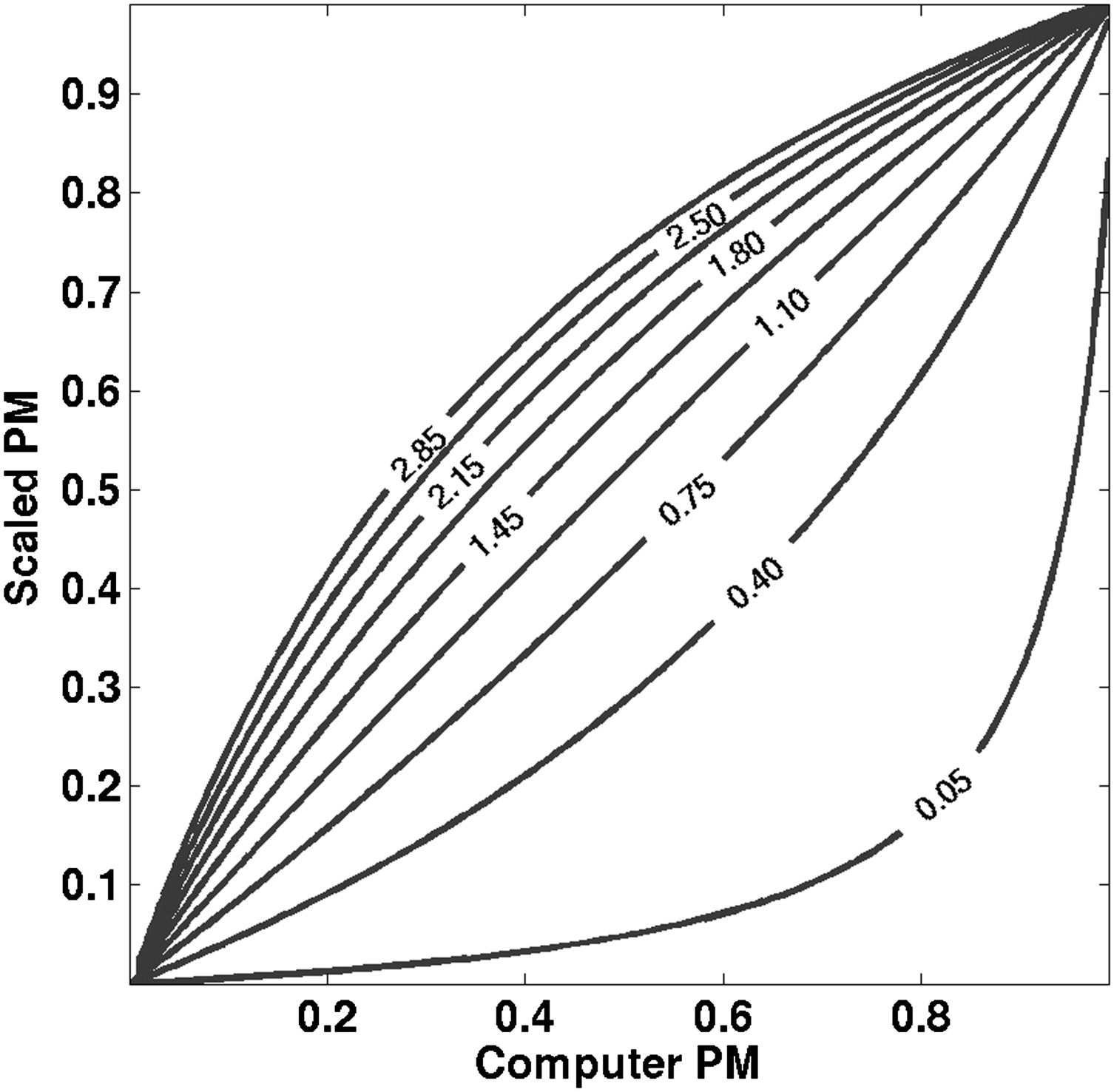
p’=κp(κ−1)p+1, p
′
=
κ
p
(
κ
−
1
)
p
+
1
,
where p is the computer PM, p′ is the scaled PM, and κ is the ratio of the scaled odds to the computer odds—that is, the ratio of the (prior) odds of malignancy when the prevalence is η scal to the odds of malignancy when the prevalence is η comp :
κ=ηscal(1−ηscal)ηcomp(1−ηcomp). κ
=
η
s
c
a
l
(
1
−
η
s
c
a
l
)
η
c
o
m
p
(
1
−
η
c
o
m
p
)
.
Get Radiology Tree app to read full this article<
Get Radiology Tree app to read full this article<
Get Radiology Tree app to read full this article<
Get Radiology Tree app to read full this article<
Get Radiology Tree app to read full this article<
Expected Utility
Get Radiology Tree app to read full this article<
E[U]=ηclin(UTP⋅TPF+UFN⋅FNF)+(1−ηclin)(UFP⋅FPF+UFN⋅TNF), E
[
U
]
=
η
c
l
i
n
(
U
T
P
⋅
T
P
F
+
U
F
N
⋅
F
N
F
)
+
(
1
−
η
c
l
i
n
)
(
U
F
P
⋅
F
P
F
+
U
F
N
⋅
T
N
F
)
,
where η clin is the clinical prevalence in the patient population of interest, whereas U TN , U FP , U TP , and U FN are the utilities associated with true negative (TN), false positive (FP), true positive (TP), and false negative (FN) decisions, respectively. (We use the word “utility” here in a general sense that connotes quantitative considerations of benefit and cost.) This expected utility reflects the clinical prevalence because we are interested in the operating point that should be used in the clinic from an expected-utility perspective. One can show ( ) that this optimal operating point occurs where the slope of the ROC curve, and therefore the likelihood ratio, equals
Ropt=(1−ηclinηclin)(UTN−UFPUTP−UFN)=RUDkclin, R
o
p
t
=
(
1
−
η
c
l
i
n
η
c
l
i
n
)
(
U
T
N
−
U
F
P
U
T
P
−
U
F
N
)
=
R
U
D
k
c
l
i
n
,
where the ratio of utility differences (RUD) and the pretest odds ( k__clin ) are given by
RUD=UTN−UFPUTP−UFNandkclin=ηclin1−ηclin, R
U
D
=
U
T
N
−
U
F
P
U
T
P
−
U
F
N
and
k
c
l
i
n
=
η
c
l
i
n
1
−
η
c
l
i
n
,
respectively. Equation 5 implies that at the optimal operating point, the post-test odds, which are the product of the likelihood ratio and the pretest odds, are a constant given by the RUD :
post-testodds =Roptkclin=RUD. post-test
odds =
R
o
p
t
k
c
l
i
n
=
R
U
D
.
Get Radiology Tree app to read full this article<
Get Radiology Tree app to read full this article<
τscal=κ∼RUDκ∼RUD+1, τ
s
c
a
l
=
κ
∼
R
U
D
κ
∼
R
U
D
+
1
,
where RUD is given by Equation 6 and the scaled-to-clinical odds ratio is given by
κ∼=ηscal(1−ηscal)ηclin(1−ηclin). κ
∼
=
η
s
c
a
l
(
1
−
η
s
c
a
l
)
η
c
l
i
n
(
1
−
η
c
l
i
n
)
.
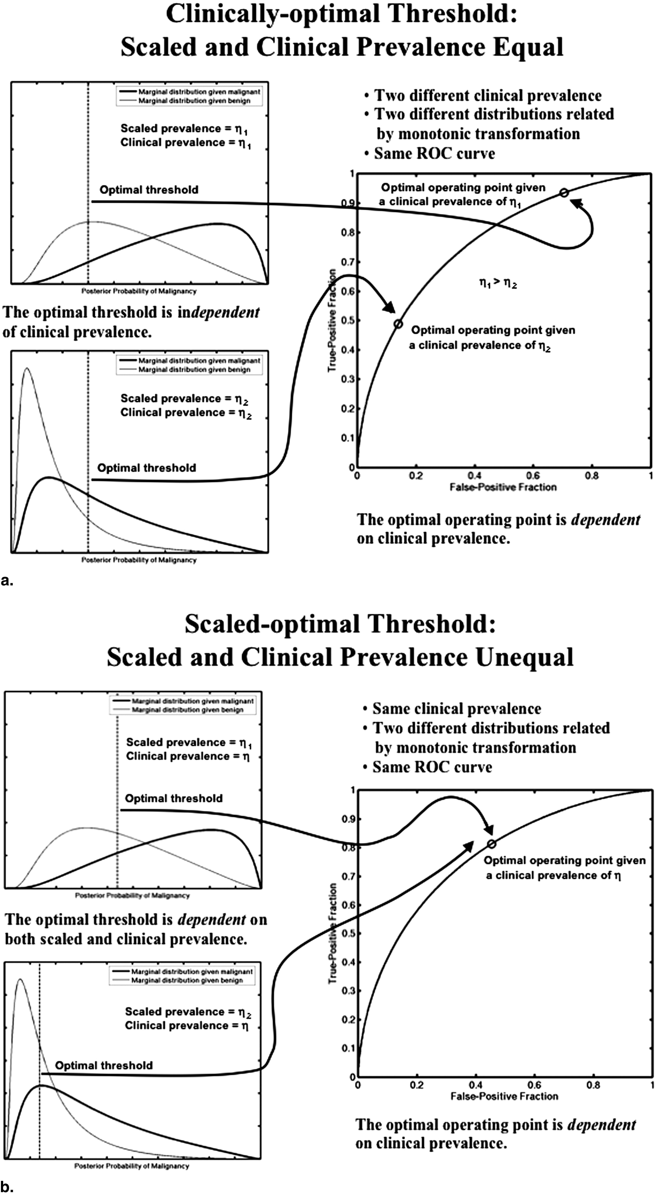
(Note the difference between the scaled-to-clinical odds ratio [Eq. 9 ], which is used to determine the scaled-optimal PM threshold, and the scaled-to-computer odds ratio [Eq. 3 ], which is used in the prevalence scaling transformation.) It is clear that when the scaled prevalence is chosen to equal the clinical prevalence (meaning that the PM has been scaled such that the prevalence reflected in the PM is the clinical prevalence and that κ˜=1 κ
˜
=
1 ), the optimal PM threshold is prevalence-independent because then it depends only on RUD
τclin=RUDRUD+1. τ
c
l
i
n
=
R
U
D
R
U
D
+
1
.
Get Radiology Tree app to read full this article<
Get Radiology Tree app to read full this article<
Get Radiology Tree app to read full this article<
Get Radiology Tree app to read full this article<
Get Radiology Tree app to read full this article<
Results
Get Radiology Tree app to read full this article<
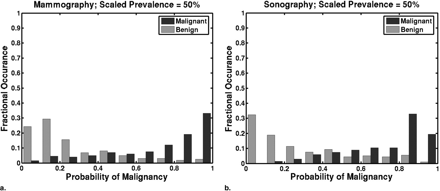
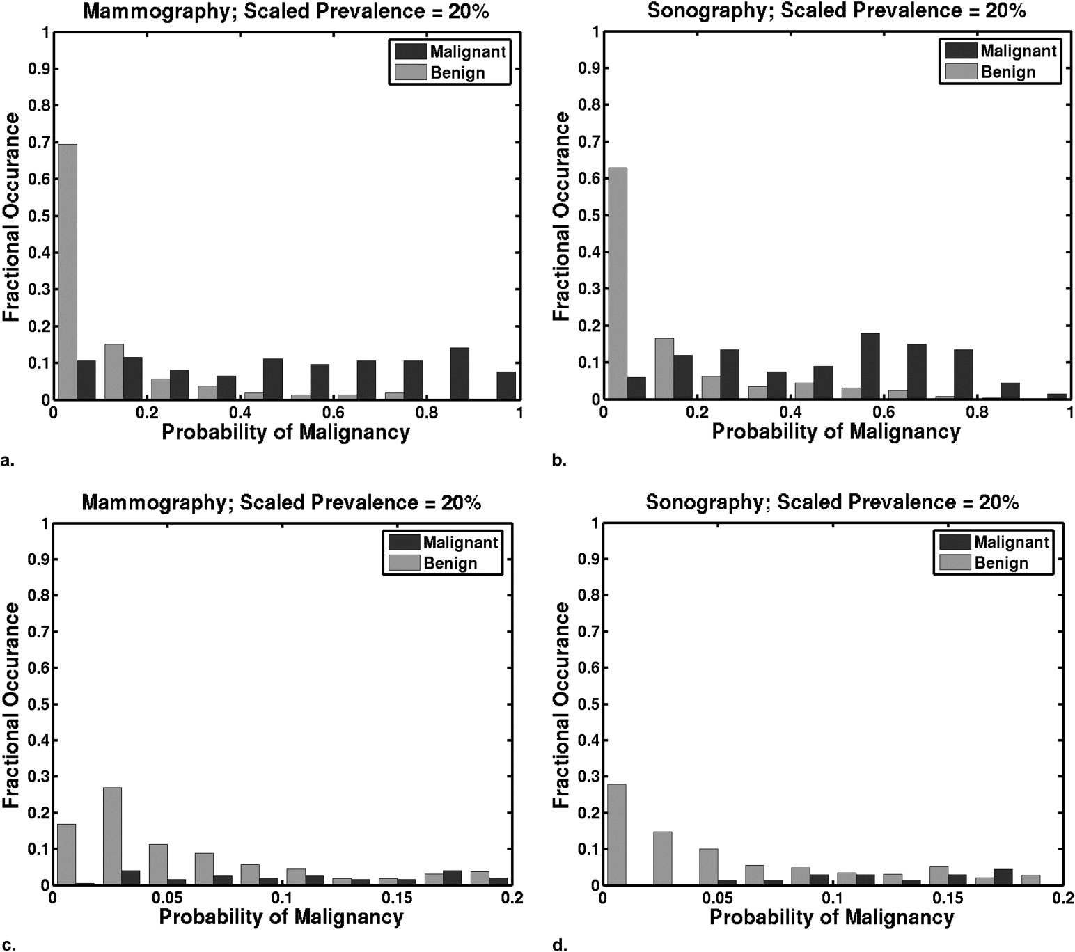
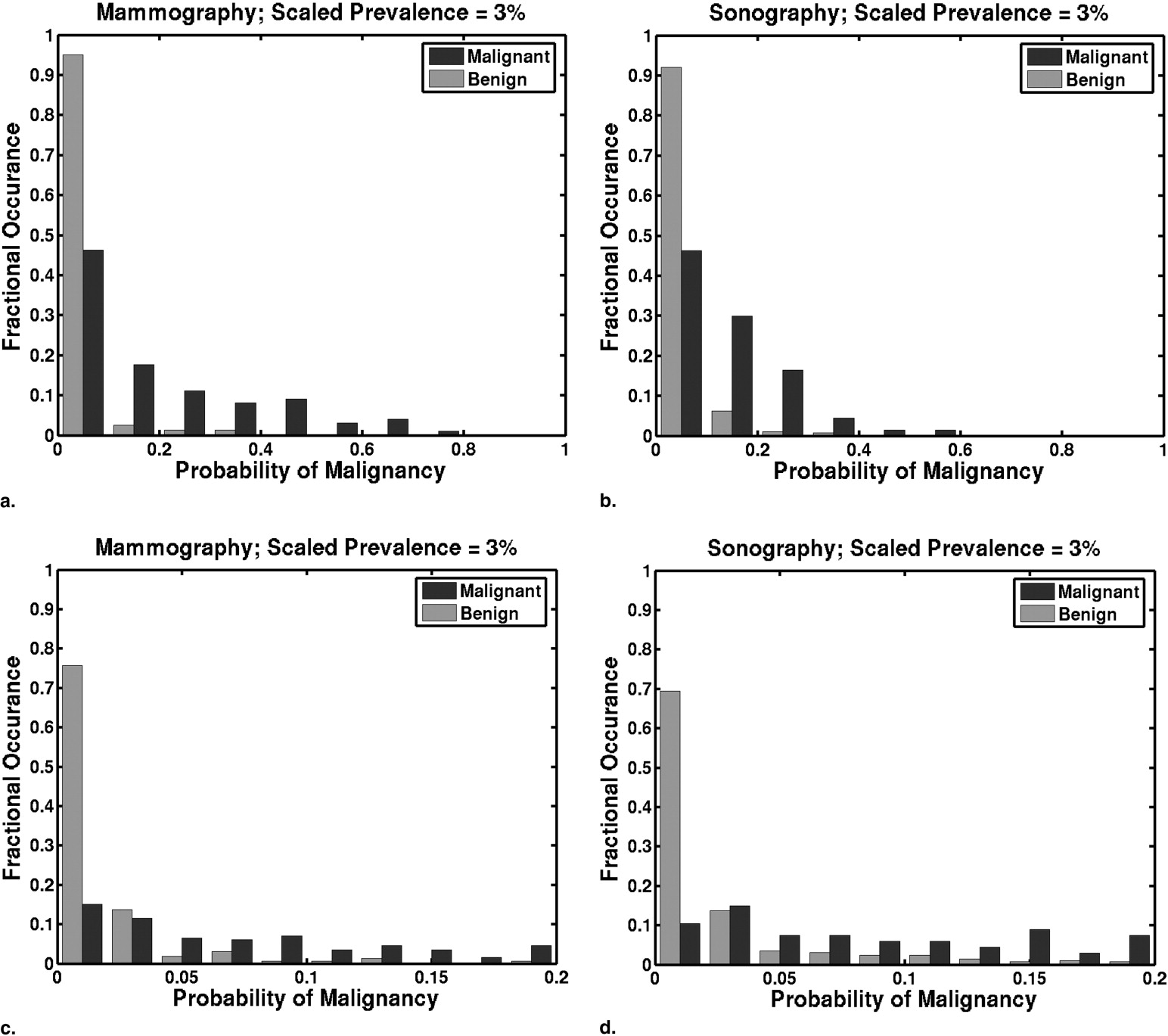
Table 1
Performance Table of the Mammographic and Sonographic Classifiers, Showing Probability of Malignancy (PM) Thresholds for Scaled Prevalences of 50%, 20%, and 3% at Various Pairs of TPF and FPF
PM Threshold as a Function of Scaled Prevalence Mammographic Classifier Performance Sonographic Classifier Performance 50% 20% 3% TPF FPF TPF FPF 0.15 0.042 0.0054 0.96 0.79 1.00 0.56 0.20 0.059 0.0077 0.95 0.62 0.99 0.49 0.25 0.077 0.010 0.93 0.52 0.97 0.43 0.30 0.097 0.013 0.88 0.39 0.96 0.37 0.35 0.12 0.016 0.84 0.30 0.91 0.34 0.40 0.14 0.020 0.80 0.33 0.90 0.30
FPF, false-positive fraction; TPF, true-positive fraction.
Table entries were computed by thresholding the PM estimates of cases in the training databases.
Get Radiology Tree app to read full this article<
Get Radiology Tree app to read full this article<
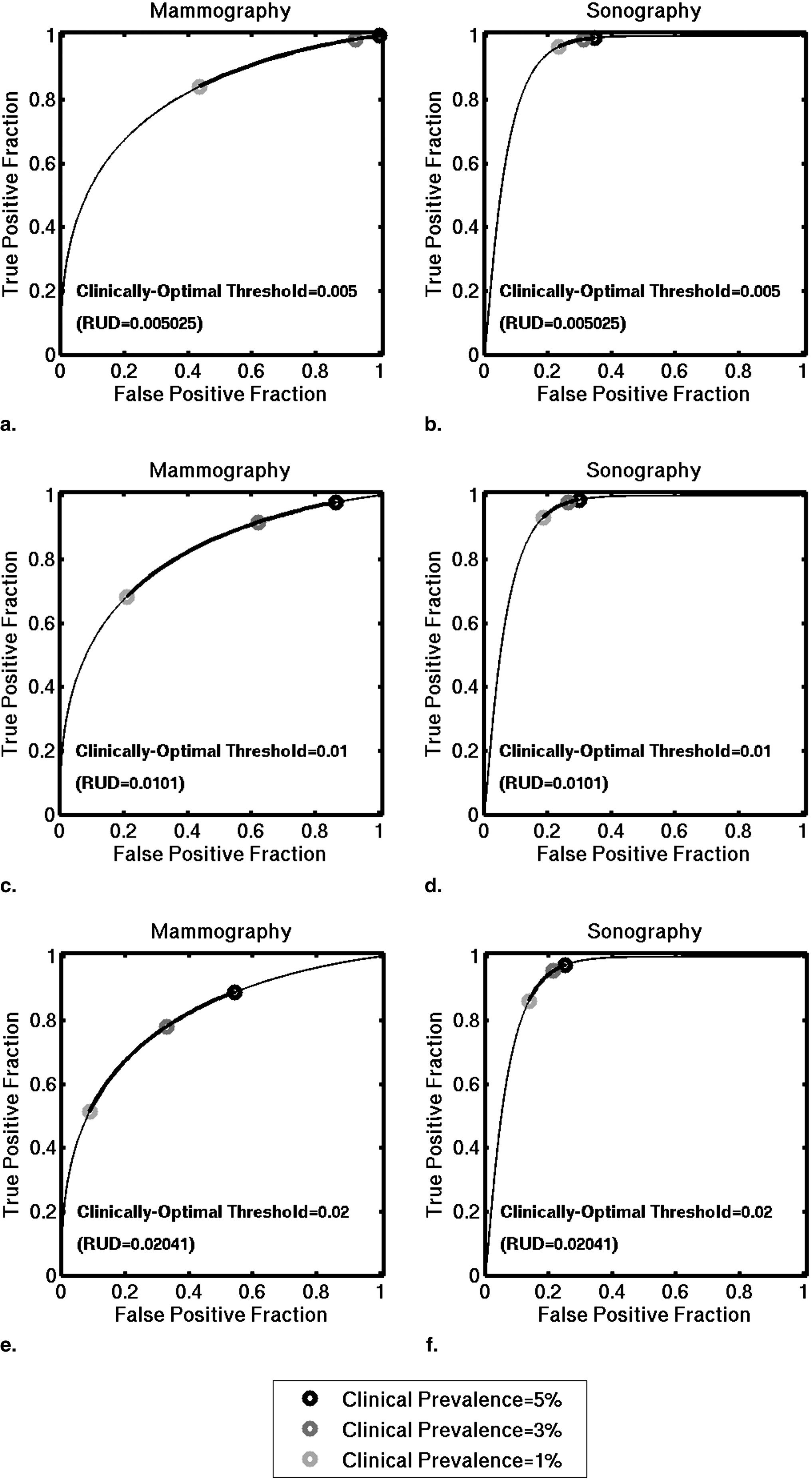
Table 2
Clinically Optimal Pairs of TPF and FPF, Assuming a Clinically Optimal Threshold of 0.02 (a threshold of 0.02 on PM Estimates that have been Scaled to Reflect Clinical Prevalence)
Clinical Prevalence Mammography Sonography Clinically Optimal Operating Point TPF Clinically Optimal Operating Point FPF Clinically Optimal Operating Point TPF Clinically Optimal Operating Point FPF 5% 0.51 0.09 0.86 0.14 4% 0.68 0.21 0.93 0.19 3% 0.78 0.33 0.95 0.22 2% 0.84 0.44 0.97 0.24 1% 0.89 0.54 0.97 0.25
Pairs of TPF and FPF were computed using the binormal parameters associated to our mammographic and sonographic classifiers evaluated on an independent multimodality database.
Get Radiology Tree app to read full this article<
Get Radiology Tree app to read full this article<
Discussion
Get Radiology Tree app to read full this article<
Get Radiology Tree app to read full this article<
Get Radiology Tree app to read full this article<
Get Radiology Tree app to read full this article<
Conclusions
Get Radiology Tree app to read full this article<
Get Radiology Tree app to read full this article<
Get Radiology Tree app to read full this article<
Get Radiology Tree app to read full this article<
Get Radiology Tree app to read full this article<
Get Radiology Tree app to read full this article<
References
1. Giger M.L., Huo Z., Vyborny C.J., Lan L., Nishikawa R.M., Rosenbourgh I.: Results of an observer study with an intelligent mammographic workstation for CAD.Peitgen H.-O.Digital mammography: IWDM 2002.2002.SpringerBerlin:pp. 297-303.
2. Giger M.L., Huo Z., Lan L., Vyborny C.J.: Intelligent search workstation for computer aided diagnosis.Lemke H.U.Inamura K.Kunio D.Vannier M.W.Farman A.G.Proceedings of Computer Assisted Radiology and Surgery (CARS) 2000.2000.ElsevierPhiladelphia:pp. 822-827.
3. Web site of the Breast Cancer Surveillance Consortium: http://breastscreening.cancer.gov/data/benchmarks/diagnostic Accessed February 26, 2008
4. Metz C.E.: Basic principles of ROC analysis. Semin Nucl Med 1978; 8: pp. 283-298.
5. Green D.M., Swets J.A.: Signal detection theory and psychophysics.1974.KriegerHuntington, NY
6. Dorfman D.D., Alf E.: Maximum-likelihood estimation of parameters of signal-detection theory and determination of confidence intervals—rating-method data. J Math Psychol 1969; 6: pp. 487-496.
7. Horsch K., Giger M.L., Vyborny C.J., Lan L., Mendelson E.B., Hendrick R.E.: Multi-modality computer-aided diagnosis for the classification of breast lesions: Observer study results on an independent clinical dataset. Radiology 2006; 240: pp. 357-368.
8. Huo Z., Giger M.L., Vyborny C.J., et. al.: Analysis of spiculation in the computerized classification of mammographic masses. Med Phys 1995; 22: pp. 1569-1579.
9. Huo Z., Giger M.L., Vyborny C.J., Woverton D.E., Schmidt R.A., Doi K.: Automated computerized classification of malignant and benign masses on digitized mammograms. Acad Radiol 1998; 5: pp. 155-168.
10. Giger M.L., Al-Hallaq H., Huo Z., et. al.: Computerized analysis of lesions in US images of the breast. Acad Radiol 1999; 6: pp. 665-674.
11. Horsch K., Giger M.L., Venta L.A., Vyborny C.J.: Automatic segmentation of breast lesions on ultrasound. Med Phys 2001; 28: pp. 1652-1659.
12. Horsch K., Giger M.L., Venta L.A., Vyborny C.J.: Computerized diagnosis of breast lesions on ultrasound. Med Phys 2002; 29: pp. 157-164.
13. Kupinski M.A., Edwards D.C., Giger M.L., Metz C.E.: Ideal observer approximation using Bayesian classification neural networks. IEEE Trans Med Imaging 2001; 20: pp. 886-899.
14. Pesce L.L., Horsch K., Metz C.E.: Estimation of the relationship between test-result values and operating points on “proper” binormal ROC curves. Presented at MIPS XII (12th meeting of the Medical Image Perception Society); Iowa City, IA, October2007.
15. Halpern E.J., Alpert M., Krieger A.M., Metz C.E., Maidment A.D.: Comparisons of ROC curves on the basis of optimal operating points. Acad Radiol 1996; 3: pp. 245-253.
16. Wagner R.F., Beam C.A., Beiden S.V.: Reader variability in mammography and its implications for expected utility over the population of readers and cases. Med Decis Making 2004; 24: pp. 561-572.
17. American College of Radiology: Breast Imaging Reporting and Data System Atlas (BI-RADS Atlas).2003.American College of RadiologyReston, VA
18. LABROC4: Website of Kurt Rossman Laboratories, Department of Radiology, University of Chicago. http://www-radiology.uchicago.edu/krl/roc_soft.htm Accessed June 10, 2004
19. Metz C.E., Herman B.A., Shen J.-H.: Maximum-likelihood estimation of ROC curves from continuously-distributed data. Statist Med 1998; 17: pp. 1033-1053.