Quantitative Measurement of Iodine Concentration in the Liver Using Abdominal C-Arm Computed Tomography

Rationale and Objectives

C-arm computed tomography is an option on a C-arm angiographic system capable of acquiring projections while rotating the C-arm around the patient and reconstructing cross-sectional images with improved contrast resolution of 5 to 10 Hounsfield units. Typical abdominal C-arm computed tomographic (CCT) images, however, exhibit artifacts with spatially varying and drifting pixel values. Considering liver tumor oncologic procedures, the aim of this study was to evaluate the accuracy of liver iodine concentration (IC) estimated from CCT images under such challenging conditions.

Materials and Methods

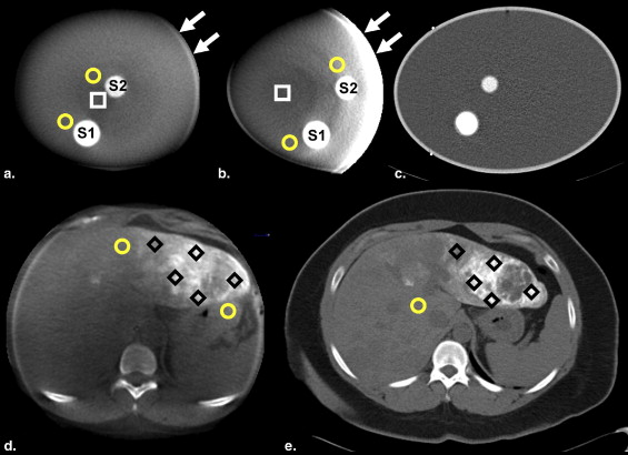
The proposed method estimates the IC in a region of interest (ROI) using pixel values of CCT images measured at the ROI and a nonenhanced background. Two approaches to measure the background value were tested: one approach, L-BG, measured a corresponding local background value near each ROI, and the other, G-BG, used one global background value for the entire object. The accuracy of estimations using CCT and computed tomographic scanners was evaluated; an elliptical cylinder water phantom with iodine solution inserts and seven patient data sets with transcatheter arterial chemoembolization were used.

Results

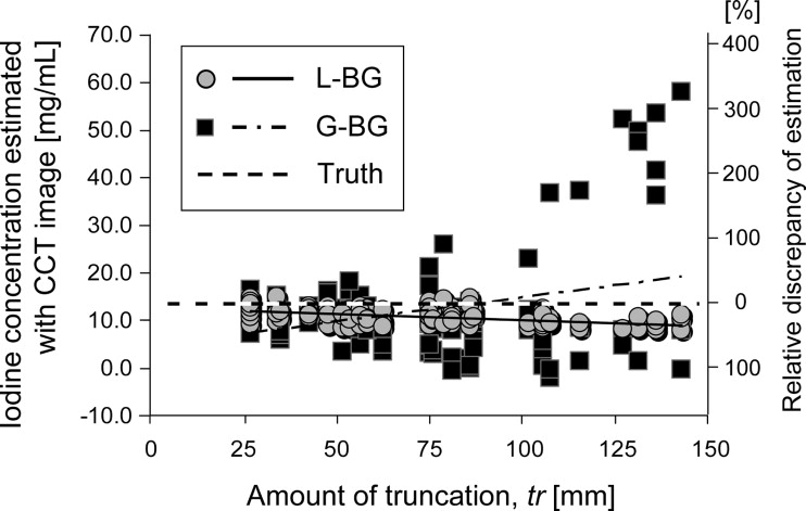
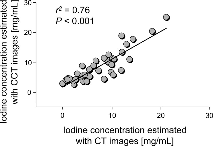
With the least “truncation” (the edge of the object being outside the field of view) of 27 mm, the IC was accurately estimated with CCT images ( n = 9; root-mean-square error [RMSE], 1.60–1.63 mg/mL; normalized RMSE, 11.8%; r 2 = 0.97; P < .001), with the true concentration ranging from 2.32 to 31.82 mg/mL. With truncations of up to 100 mm ( n = 88), the estimation by L-BG remained accurate independent of the amount of truncation (RMSE, 1.58 mg/mL; normalized RMSE, 12.5%; r 2 = 0.06; P = .02), whereas the estimation by G-BG reduced the accuracy (RMSE, 4.61 mg/mL; normalized RMSE, 34.3%; r 2 = 0.10; P = .003). Clinical data ( n = 37) showed that the estimation from CCT images using the L-BG method agreed well with that from computed tomographic images (RMSE, 2.86 mg/mL; normalized RMSE, 38.7%; r 2 = 0.76; P < .001).

Conclusion

The liver IC can be accurately estimated with abdominal CCT images.

Many image-guided interventional procedures remain subjective, even with the introduction of digital flat-panel detectors. Many interventional procedures that use x-ray images involve iodine, for example, nonionized iodine contrast agent material ( ), iodine-mixed lipiodol oil for transcatheter arterial chemoembolization (TACE) ( ), and embolic particles in an iodized solution ( ). Measuring the concentration of iodine, which is likely associated with drug concentration or blood perfusion, can lead to objective, evidence-driven procedures.

In organs, iodine is distributed three dimensionally ( ). Thus, two-dimensional projection images such as fluoroscopic or angiographic images, which show the total amount of iodine along each x-ray path, are not sufficient for accurately estimating iodine concentration (IC)—the amount of iodine per unit volume—and its spatial distribution ( ). Therefore, in this study, we used a recently developed C-arm computed tomographic (CCT) system ( ) to quantify the IC. CCT imaging is an option on C-arm angiographic systems that acquires projections while rotating the C-arm around the patient and reconstructs cross-sectional images with improved contrast resolution of 5 to 10 Hounsfield units ( ). There are two major challenges with abdominal CCT imaging: (1) to quantify the IC from a single scan and (2) to overcome the effect of artifacts unique to abdominal applications. Thus, we proposed combining two methods, each of which solves one problem. We focused on measuring the IC in the liver, because our primary clinical application was TACE for liver tumors. In principal, however, the method can be applied to other applications and organs.

Get Radiology Tree app to read full this article<

Materials and methods

Get Radiology Tree app to read full this article<

CCT System

Get Radiology Tree app to read full this article<

CT Scanner

Get Radiology Tree app to read full this article<

Phantom

Get Radiology Tree app to read full this article<

Patients

Get Radiology Tree app to read full this article<

Estimation of IC

Get Radiology Tree app to read full this article<

Truncation Correction

Get Radiology Tree app to read full this article<

Collection and Processing of the Phantom Data

Get Radiology Tree app to read full this article<

Collection and Processing of the Patient Data

Get Radiology Tree app to read full this article<

Statistical Analysis

Get Radiology Tree app to read full this article<

Results

Linearity

Get Radiology Tree app to read full this article<

Table 1

Summaries of the Estimated Iodine Concentrations with Various Iodine Densities (phantom data set 1), with Various Levels of Truncation (phantom data set 2), and with Clinical Settings (patient data)

Phantom Data Set 2 Phantom Data Set 1 ( n = 9) Truncation < 150 mm ( n = 119) Truncation < 100 mm ( n = 88) Patient Data ( n = 37) Modality and Method RMSE (mg/mL) ⁎ r 2 ∥ RMSE (mg/mL) ⁎ r 2 ∥ RMSE (mg/mL) ⁎ r 2 ∥ RMSE (mg/mL) ⁎ r 2 ‡ CCT imaging L-BG 1.63 (12.5%) 0.97 † 3.12 (23.2%) 0.25 † 1.58 (11.8%) 0.06 § 2.86 (38.7%) 0.76 † G-BG 1.60 (12.5%) 0.97 † 11.05 (82.1%) 0.09 ¶ 4.61 (34.3%) 0.10 ¶ CT imaging 0.51 (3.9%) 1.00 †

CCT, C-arm computed tomographic; CT, computed tomographic; RMSE, root-mean-square error.

Get Radiology Tree app to read full this article<

Truncation

Get Radiology Tree app to read full this article<

Patient Data

Get Radiology Tree app to read full this article<

Discussion

Get Radiology Tree app to read full this article<

Acknowledgments

Get Radiology Tree app to read full this article<

Appendix A

Get Radiology Tree app to read full this article<

μx=wIρIμ(ρ)I+wBGρBGμ(ρ)BG, μ

(

)

(

)

where w I and w BG are the relative concentration in terms of a fraction by weight, ρ I and ρ BG are the native density (in grams per cubic centimeter), and μ (ρ) I and μ (ρ) BG are the mass attenuation coefficient (in square centimeters per gram) of iodine and background material, respectively. In a case in which there is only one substance (iodine) dissolved in the background material (water or tissue), the enhancement from the background due to the iodine is related to the linear attenuation coefficients of the ROI and background by

μx= −μBG=[wIρIμ(ρ)I+wBGρBGμ(ρ)BG]−[ρBGμ(ρ)BG]=wI×[ρIμ(ρ)I−ρBGμ(ρ)BG], μ

= −

[

(

)

(

)

]

−

[

(

)

]

[

(

)

−

(

)

]

because w I = 1 − w BG . Thus, once μ x is known, w I can be estimated from a single measurement by

wI=(μx−μBG)/[ρIμ(ρ)I−ρBGμ(ρ)BG], w

(

−

)

[

(

)

−

(

)

]

where the values for the mass density of iodine, water, and liver tissue, available in the literature (20,21), are 4.93, 1.00, and 1.06 g/cm 3 , respectively. The reference x-ray photon energies of CCT and CT scanners in our study were found to be 79.0 and 78.6 keV, respectively. The mass attenuation coefficients of iodine, water, and liver tissue for CCT images were 3.713, 0.185, and 0.183 cm 2 /g, respectively. The corresponding values for CT images were 3.795, 0.185, and 0.184 cm 2 /g. To obtain the relative concentration w I , we use Equation A3 , whereby μ x and μ BG are obtained from the values of appropriate image pixels. (See Appendix C for CCT imaging and Appendix B for CT imaging.)

Get Radiology Tree app to read full this article<

IC=1000×ρI×wI. IC

1000

Get Radiology Tree app to read full this article<

Appendix B

Get Radiology Tree app to read full this article<

μx=μw×(HUX/1000+1);μBG=μw×(HUBG/1000+1), μ

(

1000

)

;

(

1000

)

where μ w = ρ w × μ (ρ)w = 0.185 cm −1 in our study. Then, we use Equation A3 to calculate w I (see Appendix A ).

Get Radiology Tree app to read full this article<

Appendix C

Get Radiology Tree app to read full this article<

fx=ax×μx+bx;fBG=aBG×μBG+bBG, f

;

where a__x , b__x and a BG , b BG are scaling and offset parameters at ROI and background, respectively. We assume that the additive offsets, b__x and b BG , are much smaller than the first terms of Equation C1 and that the scalings, a__x and a BG , are similar to each other. The ratio of μ x and μ BG can then be approximated reasonably well by

μx/μBG≈fx/fBG. μ

≈

Get Radiology Tree app to read full this article<

wI=μBG×(μx/μBG−1)/[ρIμ(ρ)I−ρBGμ(ρ)BG], w

(

−

)

[

(

)

−

(

)

]

where μ BG is the linear attenuation coefficient of the background lesion (water or liver parenchyma), which is obtained by ρ BG μ (ρ) BG , with values available in the literature.

Get Radiology Tree app to read full this article<

References

1. Gailloud P., Oishi S., Carpenter J., Murphy K.J.: Three-dimensional digital angiography: new tool for simultaneous three-dimensional rendering of vascular and osseous information during rotational angiography. AJNR Am J Neuroradiol 2004; 25: pp. 571-573.
2. Lardo A.C., Cordeiro M.A.S., Silva C., et. al.: Contrast-enhanced multidetector computed tomography viability imaging after myocardial infarction: characterization of myocyte death, microvascular obstruction, and chronic scar. Circulation 2006; 113: pp. 394-404.
3. Geschwind J.F.: Chemoembolization for hepatocellular carcinoma: where does the truth lie?. J Vasc Interv Radiol 2002; 13: pp. 991-994.
4. Ramsey D.E., Kernagis L.Y., Soulen M.C., Geschwind J.-F.H.: Chemoembolization of hepatocellular carcinoma. J Vasc Interv Radiol 2002; 13: pp. S211-S221.
5. Hong K., Khwaja A., Liapi E., Torbenson M.S., Georgiades C.S., Geschwind J.-F.H.: New intra-arterial drug delivery system for the treatment of liver cancer: preclinical assessment in a rabbit model of liver cancer. Clin Cancer Res 2006; 12: pp. 2563-2567.
6. Oto A., Tamm E.P., Szklaruk J.: Multidetector row CT of the liver. Radiol Clin North Am 2005; 43: pp. 827-848.
7. Takayasu K., Arii S., Matsuo N., et. al.: Comparison of CT findings with resected specimens after chemoembolization with iodized oil for hepatocellular carcinoma. AJR Am J Roentgenol 2000; 175: pp. 699-704.
8. Sze D.Y., Strobel N., Fahrig R., Moore T., Busque S., Frisoli J.K.: Transjugular intrahepatic portosystemic shunt creation in a polycystic liver facilitated by hybrid cross-sectional/angiographic imaging. J Vasc Interv Radiol 2006; 17: pp. 711-715.
9. Fahrig R., Dixon R., Payne T., Morin R.L., Ganguly A., Strobel N.: Dose and image quality for a cone-beam C-arm CT system. Med Phys 2006; 33: pp. 4541-4550.
10. Hirota S., Nakao N., Yamamoto S., et. al.: Cone-beam CT with flat-panel-detector digital angiography system: early experience in abdominal interventional procedures. Cardiovasc Interv Radiol 2006; 29: pp. 1034-1038.
11. Wallace M.J., Murthy R., Kamat P.P., et. al.: Impact of C-arm CT on hepatic arterial interventions for hepatic malignancies. J Vasc Interv Radiol 2007; 18: pp. 1500-1507.
12. Alvarez R.E., Macovski A.: Energy-selective reconstructions in x-ray computerised tomography. Phys Med Biol 1976; 21: pp. 733-744.
13. Kelcz F., Joseph P.M., Hilal S.K.: Noise considerations in dual energy CT scanning. Med Phys 1979; 6: pp. 418-425.
14. Gailloud P., Oishi S., Murphy K.: Three-dimensional fusion digital subtraction angiography: new reconstruction algorithm for simultaneous three-dimensional rendering of osseous and vascular information obtained during rotational angiography. AJNR Am J Neuroradiol 2005; 26: pp. 908-911.
15. van de Kraats E.B., Carelsen B., Fokkens W.J., et. al.: Direct navigation on 3D rotational x-ray data acquired with a mobile propeller C-arm: accuracy and application in functional endoscopic sinus surgery. Phys Med Biol 2005; 50: pp. 5769-5781.
16. Noo F., Clackdoyle R., Pack J.D.: A two-step Hilbert transform method for 2D image reconstruction. Phys Med Biol 2004; 49: pp. 3903-3923.
17. Feldkamp L.A., Davis L.C., Kress J.W.: Practical cone-beam algorithm. J Opt Soc Am A 1984; 1: pp. 612-619.
18. Parker D.L.: Optimal short scan convolution reconstruction for fanbeam CT. Med Phys 1982; 9: pp. 254-257.
19. Silver M.D.: A method for including redundant data in computed tomography. Med Phys 2000; 27: pp. 773-774.
20. Tissue substitutes in radiation dosimetry and measurement (ICRU Report 44).1989.International Commission on Radiation Units and MeasurementsBethesda, MD
21. Hubbell J.H., Seltzer S.M.: NIST standard reference database 126.1996.National Institute of Standards and TechnologyGaithersburg, MD
22. Barclay A.B., Eisner R.L., DiBella E.V.R.: PET thorax model database. http://www.emory.edu/CRL/abb/thoraxmodel/Contents.html Accessed September 5 2008
23. Barclay AB, Eisner RL, DiBella EVR. Construction of a thorax model database from clinical PET attenuation scans. Presented at: Annual Meeting of the Society of Nuclear Medicine, Minneapolis, MN, June 12–15, 1995.
24. Schafer D., Borgert J., Rasche V., Grass M.: Motion-compensated and gated cone beam filtered back-projection for 3-D rotational x-ray angiography. IEEE Trans Med Imaging 2006; 25: pp. 898-906.
25. Taguchi K, Kudo H. Motion compensated fan-beam reconstruction for computed tomography using derivative backprojection filtering approach. Presented at: 9th International Conference on Fully Three-Dimensional Reconstruction in Radiology and Nuclear Medicine; Lindau, Germany; July 9–13, 2007.
26. Taguchi K., Kudo H.: A simple motion tracking backprojection for a class of affine transformation. Proc SPIE 2008; 6913: pp. 66.
27. Taguchi K., Kudo H.: Motion compensated fan-beam reconstruction for nonrigid transformation. IEEE Trans Med Imaging 2008; 27: pp. 907-917.

Quantitative Measurement of Iodine Concentration in the Liver Using Abdominal C-Arm Computed Tomography

Rationale and Objectives

Materials and Methods

Results

Conclusion

Materials and methods

CCT System

CT Scanner

Phantom

Patients

Estimation of IC

Truncation Correction

Collection and Processing of the Phantom Data

Collection and Processing of the Patient Data

Statistical Analysis

Results

Linearity

Truncation

Patient Data

Discussion

Acknowledgments

Appendix A

Appendix B

Appendix C

References

Further Reading

4-D Imaging in Cerebrovascular Disorders by Using 320-Slice CT

Abstracts of Funded National Institutes of Health Grants

Breaking Bad News in the Breast Imaging Setting