Quantitative Prediction of Stone Fragility From Routine Dual Energy CT

Rationale and Objectives

Previous studies have demonstrated a qualitative relationship between stone fragility and internal stone morphology. The goal of this study was to quantify morphologic features from dual-energy computed tomography (CT) images and assess their relationship to stone fragility.

Materials and Methods

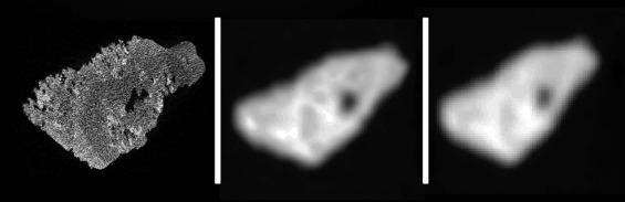
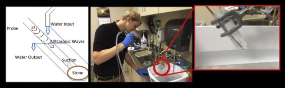
Thirty-three calcified urinary stones were scanned with micro-CT. Next, they were placed within torso-shaped water phantoms and scanned with the dual-energy CT stone composition protocol in routine use at our institution. Mixed low- and high-energy images were used to measure volume, surface roughness, and 12 metrics describing internal morphology for each stone. The ratios of low- to high-energy CT numbers were also measured. Subsequent to imaging, stone fragility was measured by disintegrating each stone in a controlled ex vivo experiment using an ultrasonic lithotripter and recording the time to comminution. A multivariable linear regression model was developed to predict time to comminution.

Results

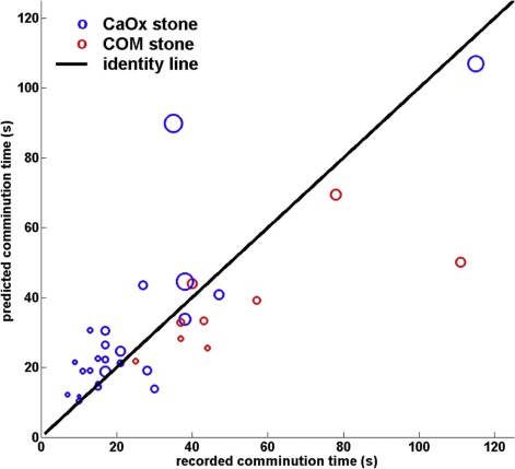
The average stone volume was 300 mm 3 (range: 134–674 mm 3 ). The average comminution time measured ex vivo was 32 seconds (range: 7–115 seconds). Stone volume, dual-energy CT number ratio, and surface roughness were found to have the best combined predictive ability to estimate comminution time (adjusted R 2 = 0.58). The predictive ability of mixed dual-energy CT images, without use of the dual-energy CT number ratio, to estimate comminution time was slightly inferior, with an adjusted R 2 of 0.54.

Conclusions

Dual-energy CT number ratios, volume, and morphologic metrics may provide a method for predicting stone fragility, as measured by time to comminution from ultrasonic lithotripsy.

Introduction

Symptomatic urinary stone disease affects approximately 900,000 persons in the United States each year, resulting in an estimated annual medical expenditure of over $1 billion in 2007 among Medicare beneficiaries alone . The prevalence of kidney stones in the United States rose by 37% between 1976–1980 and 1988–1994 in both genders . Due to the effects of global warming, it has been predicted that there could be an increase of 1.6–2.2 million lifetime cases of urinary stones by 2050 in the United States alone, as kidney stones tend to form more frequently in states where dehydration is common .

Several surgical options are available for the 10%–20% of symptomatic stone formers who fail to pass their stones spontaneously . Larger, harder kidney stones and those located in the lower pole of the kidney tend to be more easily fragmented and removed by percutaneous nephrolithotripsy (PCNL), a minimally invasive procedure whereby the stone is accessed through a small flank incision which allows direct visualization and intracorporeal ultrasonic lithotripsy for stone disruption and removal of fragments . Stone fragility, which we define as the time to comminution by a given surgical procedure, is affected by the extent of the stone burden (ie, the size and number of stones) as well as its mineral composition .

Get Radiology Tree app to read full this article<

Materials and Methods

Micro-CT Imaging

Get Radiology Tree app to read full this article<

Whole-body CT Imaging

Get Radiology Tree app to read full this article<

Texture Analysis of Stone Morphology

Get Radiology Tree app to read full this article<

coocΔx,Δy,Δz(i,j)=∑np=1∑mq=1∑or=1{1,0,ifI(p,q,r)=iandI(p+Δx,q+Δy,r+Δz)=jotherwise c

(

)

∑

{

(

)

(

)

otherwise

Get Radiology Tree app to read full this article<

TABLE 1

Haralick Features Describing Stone Internal Morphology and Features Describing Stone Surface ; cooc = co-occurrence matrix

Variable Formula Interpretation 1. Energy

∑numlevelsi=1∑numlevelsj=1cooc(i,j)2 ∑

levels

∑

levels

cooc

(

)

Uniformity of the image 2. Entropy

∑numlevelsi=1∑numlevelsj=1cooc(i,j)log10(cooc(i,j)) ∑

levels

∑

levels

cooc

(

)

(

cooc

(

)

Randomness of the image 3. Correlation

∑numlevelsi=1∑numlevelsj=1((i−μx)×(j−μy)×(cooc(i,j)/(σx×σy)) ∑

levels

∑

levels

(

−

)

(

−

)

(

cooc

(

)

(

)

Local gray level linear dependency of the image 4. Contrast

∑numlevelsi=1∑numlevelsj=1cooc(i,j)×|i−j|2 ∑

levels

∑

levels

cooc

(

)

−

Measure of local variations in the image 5. Homogeneity

∑numlevelsi=1∑numlevelsj=1cooc(i,j)|i−j|+1 ∑

levels

∑

levels

cooc

(

)

−

Local homogeneity of the image 6. Variance

∑numlevelsi=1∑numlevelsj=1((i−μx)2+(j−μy)2)×cooc(i,j) ∑

levels

∑

levels

(

−

)

(

−

)

cooc

(

)

Gray-level variability of the pixel pairs 7. Sum mean

∑numlevelsi=1∑numlevelsj=1cooc(i,j)×(i+j) ∑

levels

∑

levels

cooc

(

)

(

)

N.A. 8. Inertia

∑numlevelsi=1∑numlevelsj=1cooc(i,j)×(i+j)2 ∑

levels

∑

levels

cooc

(

)

(

)

N.A. 9. Cluster shade

∑numlevelsi=1∑numlevelsj=1(i+j−μx−μy)3cooc(i,j) ∑

levels

∑

levels

(

−

)

cooc

(

)

Skewness of the image 10. Cluster tendency

∑numlevelsi=1∑numlevelsj=1(i+j−μx−μy)4cooc(i,j) ∑

levels

∑

levels

(

−

)

cooc

(

)

Another measure of asymmetry of the image 11. Max probability

max(cooc) m

(

cooc

)

N.A. 12. Inverse variance

∑numlevelsi=1∑numlevelsj=1cooc(i,j)|i−j|2 ∑

levels

∑

levels

cooc

(

)

−

Local homogeneity of the image 13. Shape index FWHM of histogram of vertex curvatures Overall surface morphology of a stone

Get Radiology Tree app to read full this article<

Ex Vivo Analysis of Stone Fragility

Get Radiology Tree app to read full this article<

Statistical Analysis

Get Radiology Tree app to read full this article<

Results

Get Radiology Tree app to read full this article<

Univariate and Volume-adjusted Models of Stone Fragility

Get Radiology Tree app to read full this article<

TABLE 2

Association between DECT-derived Morphology Metrics and Comminution Time, Unadjusted and Adjusted for Volume

Imaging Variable Unadjusted Model Adjusted for Volume P var R 2 P var 1 P vol 2 VIF 3 R 2 adj Volumetric Volume0.00020.37\* Porosity 0.25 0.04 0.12 0.0001 1.00 0.39 Internal morphology Energy 0.24 0.04 0.09 0.0001 1.7 0.39 Entropy 0.24 0.04 0.43 0.0003 1.34 0.35 Correlation 0.34 0.03 0.98 0.0003 1.09 0.33 Contrast 0.55 0.01 0.85 0.0002 1.05 0.33 Homogeneity<0.00010.42 0.12 0.60 5.12 0.38 Variance 0.84 0 0.27 0.0001 1.10 0.36 Sum mean 0.005 0.23 0.50 0.01 1.78 0.34 Inertia 0.55 0.01 0.85 0.0002 1.05 0.33 Cluster shade 0.0002 0.36 0.23 0.15 2.98 0.37 Clusters tendency 0.15 0.07 0.37 0.0004 1.05 0.35 Max probability 0.37 0.030.04<0.00011.660.42\\ Inverse variance 0.047 0.12 0.14 0.0005 1.06 0.38 Surface morphology Shape index 0.27 0.04 0.11 0.0001 1.00 0.39 Peak curvature 0.52 0.01 0.45 0.0002 1.00 0.35 Mean curvature<0.00010.48 0.02 0.53 7.30 0.45 Dual Energy CT CT number ratio 0.25 0.040.002<0.00011.110.52\\\* HU low (90 kVp) 0.004 0.23 0.45 0.01 1.75 0.35 HU high (150 kVp)0.00010.380.020.031.520.44

CT, computed tomography.

Bold means best qualified model among those investigated.

Get Radiology Tree app to read full this article<

Best Multivariable “Single-energy” CT Models of Stone Fragility

Get Radiology Tree app to read full this article<

TABLE 3

Multivariable, Single-energy Models

Imaging Variable Adjusted for Volume and Max Probability P var 1 P vol 2 P MaxProb 3 VIF var 4 VIF vol 5 VIF MaxProb 6 R 2 adj Volumetric Volume Porosity 0.15 <0.0001 0.052 1.01 1.67 1.68 0.44 Internal morphology Energy 0.65 0.0001 0.21 10.4 1.72 10.2 0.41 Entropy 0.59 <0.0001 0.051 2.07 1.68 2.58 0.41 Correlation 0.38 <0.0001 0.03 1.26 2.08 1.93 0.42 Contrast 0.23 <0.0001 0.02 1.27 2.05 2.02 0.43 Homogeneity 0.0002 0.95 0.0001 7.36 5.25 2.39 0.63 Variance0.01<0.00010.0021.402.292.110.52 Sum mean0.0060.00030.00082.911.892.720.54\* Inertia 0.23 <0.0001 0.02 1.27 2.05 2.02 0.43 Cluster shade <0.0001 0.13 <0.0001 5.43 3.01 3.03 0.68 Clusters tendency 0.12 <0.0001 0.02 1.12 1.66 1.77 0.45 Max probability Inverse variance 1.00 0.002 0.16 2.27 3.16 3.56 0.40 Surface morphology Shape index0.02<0.00010.0081.061.731.760.50 Peak curvature 0.63 <0.0001 0.051 1.02 1.68 1.70 0.41 Mean curvature 0.003 0.81 0.006 7.49 7.49 1.71 0.57

VIF, variance inflation factor.

Bold means best qualified model among those investigated.

Get Radiology Tree app to read full this article<

Best Multivariable Dual-energy CT Models of Stone Fragility

Get Radiology Tree app to read full this article<

TABLE 4

Multivariable, Dual-energy Models

Imaging Variable Adjusted for Volume and CT Ratio P var 1 P vol 2 P CTR 3 VIF var 4 VIF vol 5 VIF CTR 6 R 2 adj Volumetric Volume Porosity 0.13 <0.0001 0.002 1.01 1.11 1.12 0.54 Internal morphology Energy 0.78 <0.0001 0.009 2.26 1.71 1.47 0.51 Entropy 0.90 <0.0001 0.003 1.41 1.38 1.18 0.51 Correlation 0.92 <0.0001 0.002 1.09 1.2 1.12 0.51 Contrast 0.84 <0.0001 0.002 1.05 1.16 1.11 0.51 Homogeneity 0.03 0.40 0.0005 5.18 5.13 1.13 0.59 Variance 0.21 <0.0001 0.002 1.1 1.22 1.11 0.53 Sum mean 0.24 0.0006 0.001 1.8 1.84 1.13 0.53 Inertia 0.84 <0.0001 0.002 1.05 1.16 1.11 0.51 Cluster shade 0.03 0.057 0.0003 3.11 2.98 1.16 0.59 Clusters tendency 0.20 <0.0001 0.001 1.05 1.15 1.12 0.53 Max probability 0.70 <0.0001 0.02 2.57 1.7 1.72 0.51 Inverse variance 0.87 <0.0001 0.006 1.34 1.31 1.41 0.51 Surface morphology Shape index0.03<0.00010.00061.011.121.120.58\* Peak curvature 0.56 <0.0001 0.002 1.01 1.12 1.12 0.51 Mean curvature 0.03 0.84 0.003 7.53 7.91 1.15 0.58 DECT CT number ratio HU low (90 kVp)0.040.0010.00031.921.761.220.57 HU high (150 kVp)0.040.0010.0031.571.741.150.57

CT, computed tomography.

Bold means best qualified model among those investigated.

Get Radiology Tree app to read full this article<

Discussion

Get Radiology Tree app to read full this article<

Conclusions

Get Radiology Tree app to read full this article<

Acknowledgments

Get Radiology Tree app to read full this article<

Supplementary Data

Get Radiology Tree app to read full this article<

Figure S1

Get Radiology Tree app to read full this article<

References

1. Pearle M.S., Calhoun E.A., Curhan G.C.: Urologic diseases in America project: urolithiasis. J Urol 2005; 173: pp. 848-857.
2. Litwin M., Saigal C.: Economic impact of urologic disease.Litwin M.S.Saigal C.S.Urologic diseases in America.2012.US Government Printing OfficeWashington, DC:pp. 494. US Department of Health and Human Services, Public Health Service, National Institutes of Health, National Institute of Diabetes and Digestive and Kidney Diseases
3. Stamatelou K.K., Francis M.E., Jones C.A., et. al.: Time trends in reported prevalence of kidney stones in the United States: 1976–1994. Kidney Int 2003; 63: pp. 1817-1823.
4. Brikowski T.H., Lotan Y., Pearle M.S.: Climate-related increase in the prevalence of urolithiasis in the United States. Proc Natl Acad Sci USA 2008; 105: pp. 9841-9846.
5. Auge B.K., Preminger G.M.: Surgical management of urolithiasis. Endocrinol Metab Clin North Am 2002; 31: pp. 1065-1082.
6. Lingeman J., Newmark J., Wong M.: Classification and management of staghorn calculi. Controversies in endourology.1995.SaundersPhiladelphiapp. 136-144.
7. Williams J.C., Saw K.C., Paterson R.F., et. al.: Variability of renal stone fragility in shock wave lithotripsy. Urology 2003; 61: pp. 1092-1096. discussion 7
8. Coursey C.A., Casalino D.D., Remer E.M., et. al.: ACR Appropriateness Criteria® acute onset flank pain–suspicion of stone disease. Ultrasound Q 2012; 28: pp. 227-233.
9. Fulgham P.F., Assimos D.G., Pearle M.S., et. al.: Clinical effectiveness protocols for imaging in the management of ureteral calculous disease: AUA technology assessment. J Urol 2013; 189: pp. 1203-1213.
10. Vrtiska T.J., Takahashi N., Fletcher J.G., et. al.: Genitourinary applications of dual-energy CT. AJR Am J Roentgenol 2010; 194: pp. 1434-1442.
11. Stolzmann P., Kozomara M., Chuck N., et. al.: In vivo identification of uric acid stones with dual-energy CT: diagnostic performance evaluation in patients. Abdom Imaging 2010; 35: pp. 629-635.
12. Primak A.N., Fletcher J.G., Vrtiska T.J., et. al.: Noninvasive differentiation of uric acid versus non-uric acid kidney stones using dual-energy CT. Acad Radiol 2007; 14: pp. 1441-1447.
13. Yu L., Liu X., Leng S., et. al.: Radiation dose reduction in computed tomography: techniques and future perspective. Imaging Med 2009; 1: pp. 65-84.
14. Boll D.T., Patil N.A., Paulson E.K., et. al.: Renal stone assessment with dual-energy multidetector CT and advanced postprocessing techniques: improved characterization of renal stone composition–pilot study. Radiology 2009; 250: pp. 813-820.
15. Qu M., Ramirez-Giraldo J.C., Leng S., et. al.: Dual-energy dual-source CT with additional spectral filtration can improve the differentiation of non-uric acid renal stones: an ex vivo phantom study. AJR Am J Roentgenol 2011; 196: pp. 1279-1287.
16. Williams J.C., Hameed T., Jackson M.E., et. al.: Fragility of brushite stones in shock wave lithotripsy: absence of correlation with computerized tomography visible structure. J Urol 2012; 188: pp. 996-1001.
17. Kim S.C., Burns E.K., Lingeman J.E., et. al.: Cystine calculi: correlation of CT-visible structure, CT number, and stone morphology with fragmentation by shock wave lithotripsy. Urol Res 2007; 35: pp. 319-324.
18. Zarse C.A., Hameed T.A., Jackson M.E., et. al.: CT visible internal stone structure, but not Hounsfield unit value, of calcium oxalate monohydrate (COM) calculi predicts lithotripsy fragility in vitro. Urol Res 2007; 35: pp. 201-206.
19. Zarse C.A., McAteer J.A., Sommer A.J., et. al.: Nondestructive analysis of urinary calculi using micro computed tomography. BMC Urol 2004; 4: pp. 15.
20. Williams J.C., McAteer J.A., Evan A.P., et. al.: Micro-computed tomography for analysis of urinary calculi. Urol Res 2010; 38: pp. 477-484.
21. Duan X., Wang J., Qu M., et. al.: Kidney stone volume estimation from computerized tomography images using a model based method of correcting for the point spread function. J Urol 2012; 188: pp. 989-995.
22. Haralick R.M., Shanmugam K., Dinstein I.H.: Textural features for image classification. IEEE Trans Syst Man Cybern 1973; SMC-3: pp. 610-621.
23. Duan X., Qu M., Wang J., et. al.: Differentiation of calcium oxalate monohydrate and calcium oxalate dihydrate stones using quantitative morphological information from micro-computerized and clinical computerized tomography. J Urol 2013; 189: pp. 2350-2356.
24. Weiss N.A., Weiss C.A.: Introductory statistics.7th ed.2005.Addison-Wesley Publishing CompanyBoston
25. R Foundation : What is R? Introduction to R. Available at: https://www.r-project.org/about.html Accessed December 14, 2015
26. Krambeck A.E., Lingeman J.E., McAteer J.A., et. al.: Analysis of mixed stones is prone to error: a study with US laboratories using micro CT for verification of sample content. Urol Res 2010; 38: pp. 469-475.
27. Michel M.S., Trojan L., Rassweiler J.J.: Complications in percutaneous nephrolithotomy. Eur Urol 2007; 51: pp. 899-906. discussion
28. Dogan H.S., Sahin A., Cetinkaya Y., et. al.: Antibiotic prophylaxis in percutaneous nephrolithotomy: prospective study in 81 patients. J Endourol 2002; 16: pp. 649-653.
29. El-Assmy A.M., Shokeir A.A., El-Nahas A.R., et. al.: Outcome of percutaneous nephrolithotomy: effect of body mass index. Eur Urol 2007; 52: pp. 199-205.
30. Kang D.E., Maloney M.M., Haleblian G.E., et. al.: Effect of medical management on recurrent stone formation following percutaneous nephrolithotomy. J Urol 2007; 177: pp. 1785-1789.

Quantitative Prediction of Stone Fragility From Routine Dual Energy CT

Rationale and Objectives

Materials and Methods

Results

Conclusions

Introduction

Materials and Methods

Micro-CT Imaging

Whole-body CT Imaging

Texture Analysis of Stone Morphology

Ex Vivo Analysis of Stone Fragility

Statistical Analysis

Results

Univariate and Volume-adjusted Models of Stone Fragility

Best Multivariable “Single-energy” CT Models of Stone Fragility

Best Multivariable Dual-energy CT Models of Stone Fragility

Discussion

Conclusions

Acknowledgments

Supplementary Data

References

Further Reading

A Guide to Writing Academic Portfolios for Radiologists

A Review of Supplemental Screening Ultrasound for Breast Cancer

Associations Between Academic Rank and Advanced Bibliometric Indices Among United States Academic Radiologists