
Rationale and Objectives
Alveolar oxygen tension (P ao 2 ) is sensitive to the interplay between local ventilation, perfusion, and alveolar-capillary membrane permeability, and thus reflects physiologic heterogeneity of healthy and diseased lung function. Several hyperpolarized helium ( 3 He) magnetic resonance imaging (MRI)-based P ao 2 mapping techniques have been reported, and considerable effort has gone toward reducing P ao 2 measurement error. We present a new P ao 2 imaging scheme, using parallel accelerated MRI, which significantly reduces measurement error.
Materials and Methods
The proposed P ao 2 mapping scheme was computer-simulated and was tested on both phantoms and five human subjects. Where possible, correspondence between actual local oxygen concentration and derived values was assessed for both bias (deviation from the true mean) and imaging artifact (deviation from the true spatial distribution).
Results
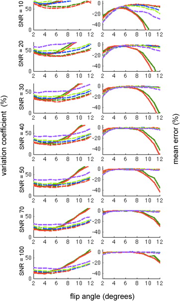
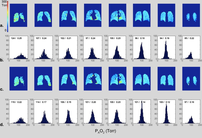
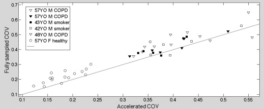
Phantom experiments demonstrated a significantly reduced coefficient of variation using the accelerated scheme. Simulation results support this observation and predict that correspondence between the true spatial distribution and the derived map is always superior using the accelerated scheme, although the improvement becomes less significant as the signal-to-noise ratio increases. Paired measurements in the human subjects, comparing accelerated and fully sampled schemes, show a reduced P ao 2 distribution width for 41 of 46 slices.
Conclusion
In contrast to proton MRI, acceleration of hyperpolarized imaging has no signal-to-noise penalty; its use in P ao 2 measurement is therefore always beneficial. Comparison of multiple schemes shows that the benefit arises from a longer time-base during which oxygen-induced depolarization modifies the signal strength. Demonstration of the accelerated technique in human studies shows the feasibility of the method and suggests that measurement error is reduced here as well, particularly at low signal-to-noise levels.
Hyperpolarized (HP) helium ( 3 He) magnetic resonance imaging (MRI) is an attractive method for imaging pulmonary disorders because of established contrast techniques that impose sensitivity to airway disease , alveolar integrity , lung perfusion , and the regional alveolar partial pressure of oxygen (P ao 2 ). The latter parameter is closely related to the local ventilation-perfusion ratio , and the distribution of P ao 2 values reflects the physiologic heterogeneity of the lung. Measured distributions of values, however, are also sensitive to noise, the application of radiofrequency (RF) pulses, and potentially to gas redistribution within the lung during the measurement . To use the P A O 2 map as a reliable biomarker for lung disease diagnosis or assessment, the relative contribution of these confounding factors needs to be understood and the effects on the measurement must be minimized.
Several related P ao 2 measurement methods using HP 3 He MRI have been introduced over the past decade . In all of these techniques, the regional P ao 2 level is calculated from the oxygen (O 2 )-induced 3 He depolarization rate. To achieve an acceptable image signal-to-noise ratio (SNR), however, sufficient RF power must be applied so that its depolarization effect cannot be neglected. Accurate separation of the two types of depolarization mechanisms holds the key to reliable P ao 2 mapping. This separation can be accomplished by acquiring identical image sets in which only the RF power is varied , although more efficient use of available gas and superior immunity to subject motion can be achieved by using a variable interscan acquisition delay scheme during a single breath-hold . Optimization of the timing scheme has been undertaken, and the effect on breath-hold duration and extracted P ao 2 uncertainty has been well studied .
Get Radiology Tree app to read full this article<
Get Radiology Tree app to read full this article<
Background
Theory
Get Radiology Tree app to read full this article<
1T1=0.45(299T)0.42[O2] 1
T
1
=
0.45
(
299
T
)
0.42
[
O
2
]
where T 1 , T , and [O 2 ] are measured in seconds, K, and amagats, respectively . At body temperature, 310 K, Equation 1 yields:
T1=ξ/pO2 T
1
=
ξ
/
p
O
2
where ξ = 1950 Torr · s.
Get Radiology Tree app to read full this article<
Get Radiology Tree app to read full this article<
Mn=M0cosnNPE(α)×exp[−PAO2⋅tn(k)/ζ] M
n
=
M
0
cos
n
N
P
E
(
α
)
×
exp
[
−
P
AO
2
⋅
t
n
(
k
)
/
ζ
]
where M 0 and M n are the magnetization levels of the region of interest in the initial and n -th image, respectively, and t__n ( k ) is the start time of the n- th acquisition of the k -th slice. We note that alveolar oxygen tension will decrease slowly (and approximately linearly ) during the breath-hold because of oxygen uptake into the blood. We do not formally include this effect in Equation 3 ; P ao 2 in this expression therefore refers to the average oxygen tension between t = 0 and t = t__n . To very good approximation, we may consider it to refer to the average P ao 2 during the breath-hold.
Get Radiology Tree app to read full this article<
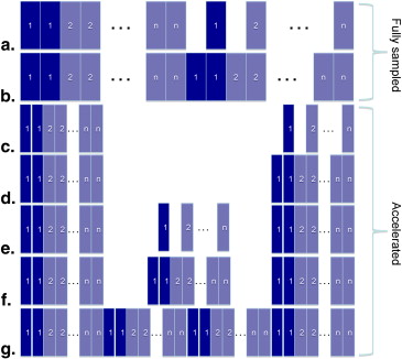
Timing Scheme of P ao 2 Acquisition
Get Radiology Tree app to read full this article<
Get Radiology Tree app to read full this article<
Get Radiology Tree app to read full this article<
Parallel Accelerated Imaging for Hyperpolarized Gas
Get Radiology Tree app to read full this article<
Sn(kx,ky)=∬dxdyCn(x,y)M0(x,y)exp(−jkxx−jkyy) S
n
(
k
x
,
k
y
)
=
∬
d
x
d
y
C
n
(
x
,
y
)
M
0
(
x
,
y
)
exp
(
−
j
k
x
x
−
j
k
y
y
)
in which M 0 represents the initial longitudinal magnetization, C__n and S__n are the coil sensitivity profile and sampled k -space signal of the n- th coil, respectively, and k x = γG x t x and k y = γG y t y are the phase-encoding steps achieved by applying magnetic field gradient G for time t . The number of gradient phase–encoding steps can be reduced by simultaneous acquisition of spatial harmonics with a sinusoidal coil sensitivity profile that is approximated by a linearly combined surface coil array. In such a case, as shown in Equations 5 and 6 , the spatially varying coil sensitivity causes shifts in k -space and is used as an alternate way of phase encoding that is otherwise produced only by magnetic field gradients.
C(x,y)=C0cos(Δkxx)+jC0sin(Δkxx)=C0exp(jΔkxx) C
(
x
,
y
)
=
C
0
cos
(
Δ
k
x
x
)
+
j
C
0
sin
(
Δ
k
x
x
)
=
C
0
exp
(
j
Δ
k
x
x
)
Sn(kx,ky)=∬dxdyCn(x,y)M0(x,y)exp(−jkxx−jkyy)=∬dxdyCn0M0(x,y)exp(−j(kx−Δkx)x−jkyy) S
n
(
k
x
,
k
y
)
=
∬
d
x
d
y
C
n
(
x
,
y
)
M
0
(
x
,
y
)
exp
(
−
j
k
x
x
−
j
k
y
y
)
=
∬
d
x
d
y
C
n
0
M
0
(
x
,
y
)
exp
(
−
j
(
k
x
−
Δ
k
x
)
x
−
j
k
y
y
)
When compared to other k -space acquisition schemes , generalized autocalibrating partially parallel acquisitions (GRAPPA) is noteworthy in that it minimizes SNR loss arising from partial cancellation of the individual coil’s signal. For each of the m coils in the receive array, k -space sampling is specified by an acceleration factor and number of autocalibration lines, chosen from the fully sampled set near k = 0. The full k -space and its corresponding uncombined image are then generated and the final image is reconstructed by combining all of the m individual images.
Get Radiology Tree app to read full this article<
Get Radiology Tree app to read full this article<
Sn(kx,ky)=∑Nx=1∑Ny=1M0(x,y)sin(α)Cn(x,y)exp(−(kx−1)TRT1)×coskx−1(α)exp(j2π(kx+ky)N) S
n
(
k
x
,
k
y
)
=
∑
x
=
1
N
∑
y
=
1
N
M
0
(
x
,
y
)
sin
(
α
)
C
n
(
x
,
y
)
exp
(
-
(
k
x
-
1
)
TR
T
1
)
×
cos
k
x
−
1
(
α
)
exp
(
j
2
π
(
k
x
+
k
y
)
N
)
where M 0 (x,y) is the initial total magnetization, C n (x,y) is the coil sensitivity, α is the flip-angle, e−(kx−1)TR/T1 e
−
(
k
x
−
1
)
T
R
/
T
1 is the nonrecoverable T 1 relaxation by oxygen, coskx−1(α) cos
k
x
−
1
(
α
) is the nonrecoverable decay by RF pulses, ej2π(kx+ky)/N e
j
2
π
(
k
x
+
k
y
)
/
N is the phase-encoding term, and N is the total phase-encoding steps.
Get Radiology Tree app to read full this article<
Materials and methods
P ao 2 Acquisition Simulations and Error Estimation
Get Radiology Tree app to read full this article<
Get Radiology Tree app to read full this article<
Get Radiology Tree app to read full this article<
μ−μactual=1N∑Ni=1pO2i,measured−pO2i,actual μ
−
μ
a
c
t
u
a
l
=
1
N
∑
i
=
1
N
p
O
2
i
,
m
e
a
s
u
r
e
d
−
p
O
2
i
,
a
c
t
u
a
l
VC=1N∑Ni=1(pO2i,measured−pO2i,actual−(μ−μactual))2(pO2i,actual)2−−−−−−−−−−−−−−−−−−−−−−−−−−−−−√ VC
=
1
N
∑
i
=
1
N
(
p
O
2
i
,
m
e
a
s
u
r
e
d
−
p
O
2
i
,
a
c
t
u
a
l
−
(
μ
−
μ
a
c
t
u
a
l
)
)
2
(
p
O
2
i
,
a
c
t
u
a
l
)
2
Get Radiology Tree app to read full this article<
Get Radiology Tree app to read full this article<
Phantom Experiments
Get Radiology Tree app to read full this article<
Get Radiology Tree app to read full this article<
Human Experiments
Get Radiology Tree app to read full this article<
Get Radiology Tree app to read full this article<
Get Radiology Tree app to read full this article<
Get Radiology Tree app to read full this article<
Get Radiology Tree app to read full this article<
Results
Simulation
Get Radiology Tree app to read full this article<
Get Radiology Tree app to read full this article<
Get Radiology Tree app to read full this article<
Get Radiology Tree app to read full this article<
Get Radiology Tree app to read full this article<
Get Radiology Tree app to read full this article<
Phantom Experiment Results
Get Radiology Tree app to read full this article<
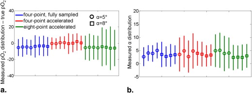
Table 1
Compete Summary of Tedlar Bag Phantom Studies
Mean p o 2 Estimation Error (%) p o 2 Map Variation Coefficient (%) α = 5 Fully sampled Accelerated Accelerated Fully sampled Accelerated Accelerated 4-point 8-point 4-point 8-point Trial 1 −5.28 −0.31 −5.55 10.18 7.18 14.57 Trial 2 −4.58 −0.48 −4.94 11.73 6.33 16.37 Trial 3 −4.62 0.58 −5.07 9.17 7.44 14.71 Trial 4 −5.50 0.70 −5.62 9.35 7.58 14.51 Group mean −5.00 0.12 −5.23 10.11 7.13 15.04 α = 8 Fully sampled Accelerated Accelerated Fully sampled Accelerated Accelerated 4-point 8-point 4-point 8-point Trial 1 −3.86 −0.44 −4.39 13.37 12.54 23.50 Trial 2 −3.30 0.04 −4.96 11.36 10.91 21.81 Trial 3 −3.38 2.05 −6.17 12.36 10.86 26.53 Trial 4 −3.94 0.25 −5.94 11.30 8.71 22.07 Group mean −3.62 0.48 −5.37 12.10 10.76 23.48
Shaded columns correspond to metrics derived from fully sampled images; unshaded columns correspond to accelerated images.
Get Radiology Tree app to read full this article<
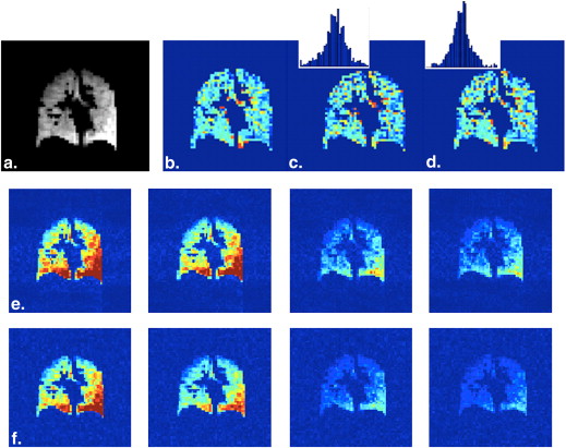
Human Experiments Results
Get Radiology Tree app to read full this article<
Get Radiology Tree app to read full this article<
Discussion
Get Radiology Tree app to read full this article<
Timing Scheme Optimization
Get Radiology Tree app to read full this article<
Get Radiology Tree app to read full this article<
Get Radiology Tree app to read full this article<
Qualitative Discussion of Human Imaging Results
Get Radiology Tree app to read full this article<
Get Radiology Tree app to read full this article<
Diffusion and the Distribution of Observed P ao 2 Values
Get Radiology Tree app to read full this article<
Get Radiology Tree app to read full this article<
Routine or Clinical Use
Get Radiology Tree app to read full this article<
Conclusion
Get Radiology Tree app to read full this article<
Acknowledgment
Get Radiology Tree app to read full this article<
References
1. Santyr G.E., Lam W.W., Parra-Robles J.M., et. al.: Hyperpolarized noble gas magnetic resonance imaging of the animal lung: approaches and applications. J Appl Phys 2009; 10: pp. 102004.
2. Emami K., Kadlecek S.J., Woodburn J.M., et. al.: Improved technique for measurement of regional fractional ventilation by hyperpolarized 3 He MRI. Magn Reson Med 2010; 63: pp. 137-150.
3. Yablonskiy D.A., Sukstanskii A.L., Woods J.C., et. al.: Quantification of lung microstructure with hyperpolarized 3 He diffusion MRI. J Appl Phys 2009; 107: pp. 1258-1265.
4. van Beek E.J., Wild J.M., Kauczor H.-U., et. al.: Functional MRI of the lung using hyperpolarized 3-helium gas. J MRI 2004; 20: pp. 540-554.
5. Rizi R.R., Baumgardner J.E., Ishii M., et. al.: Determination of regional V A /Q by hyperpolarized 3 He MRI. Magn Reson Med 2004; 52: pp. 65-72.
6. Kadlecek S., Mongkolwisetwara P., Xin Y., et. al.: Regional determination of oxygen uptake in rodent lungs using hyperpolarized gas and an analytical treatment of intrapulmonary gas redistribution. NMR Biomed 2011; 24: pp. 1253-1263.
7. Deninger A.J., Eberle B., Ebert M., et. al.: Quantification of regional intrapulmonary oxygen partial pressure evolution during apnea by 3He MRI. J Magn Res 1999; 141: pp. 207-216.
8. Fischer M.C., Spector Z.Z., Ishii M., et. al.: Single-acquisition sequence for the measurement of oxygen partial pressure by hyperpolarized gas MRI. Magn Reson Med 2004; 52: pp. 766-773.
9. Fischer M.C., Kadlecek S., Yu J.S., et. al.: Measurements of regional alveolar oxygen pressure using hyperpolarized 3 He MRI. Acad Radiol 2005; 12: pp. 1430-1439.
10. Yu J., Ishii M., Law M., et. al.: Optimization of scan parameters in pulmonary partial pressure oxygen measurement by hyperpolarized 3 He MRI. Magn Reson Med 2008; 59: pp. 124-131.
11. Miller G.W., Mugler J.P., Altes T.A., et. al.: A short-breath-hold technique for lung pO 2 mapping with 3 He MRI. Magn Reson Med 2010; 63: pp. 127-136.
12. Sodickson D.K., Manning W.J.: Simultaneous acquisition of spatial harmonics (SMASH): fast imaging with radiofrequency coil arrays. Magn Reson Med 1997; 38: pp. 591-603.
13. Pruessmann K.P., Weiger M., Scheidegger M.B., et. al.: SENSE: sensitivity encoding for fast MRI. Magn Reson Med 1999; 42: pp. 952-962.
14. Griswold M.A., Jakob P.M., Heidemann R.M., et. al.: Generalized autocalibrating partially parallel acquisitions (GRAPPA). Magn Reson Med 2002; 47: pp. 1202-1210.
15. Vasanawala S.S., Yu H., Shimakawa A., et. al.: A flexible 32-channel receive array combined with a homogeneous transmit coil for human lung imaging with hyperpolarized (3) He at 1.5 T. Magn Reson Med 2012; 67: pp. 183-190.
16. Lee R.F., Johnson G., Grossman R.I., et. al.: Advantages of parallel imaging in conjunction with hyperpolarized helium—a new approach to MRI of the lung. Magn Reson Med 2006; 55: pp. 1132-1141.
17. Saam B., Happer W., Middleton H.: Nuclear relaxation of 3 He in the presence of O 2 . Phys Rev A 1995; 52: pp. 862-865.
18. Hamedani H., Kadlecek S.J., Emami K., et. al.: A multislice single breath-hold scheme for imaging alveolar oxygen tension in humans. Magn Reson Med 2012; 67: pp. 1332-1345.
19. Yu J., Rajaei S., Ishii M., et. al.: Measurement of pulmonary partial pressure of oxygen and oxygen depletion rate with hyperpolarized helium-3 MRI: a preliminary reproducibility study on pig model. Acad Radiol 2008; 15: pp. 702-712.
20. Wild J.M., Fichele S., Woodhouse N., et. al.: 3D volume-localized pO 2 measurement in the human lung with 3 He MRI. Magn Reson Med 2005; 53: pp. 1055-1064.