Registering Histologic and MR Images of Prostate for Image-based Cancer Detection

Rationale and Objectives

Needle biopsy is currently the only way to confirm prostate cancer. To increase prostate cancer diagnostic rate, needles are expected to be deployed at suspicious cancer locations. High-contrast magnetic resonance (MR) imaging provides a powerful tool for detecting suspicious cancerous tissues. To do this, MR appearances of cancerous tissue should be characterized and learned from a sufficient number of prostate MR images with known cancer information. However, ground-truth cancer information is only available in histologic images. Therefore it is necessary to warp ground-truth cancerous regions in histological images to MR images by a registration procedure. The objective of this article is to develop a registration technique for aligning histological and MR images of the same prostate.

Material and Methods

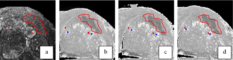
Five pairs of histological and T2-weighted MR images of radical prostatectomy specimens are collected. For each pair, registration is guided by two sets of correspondences that can be reliably established on prostate boundaries and internal salient bloblike structures of histologic and MR images.

Results

Our developed registration method can accurately register histologic and MR images. It yields results comparable to manual registration, in terms of landmark distance and volume overlap. It also outperforms both affine registration and boundary-guided registration methods.

Conclusions

We have developed a novel method for deformable registration of histologic and MR images of the same prostate. Besides the collection of ground-truth cancer information in MR images, the method has other potential applications. An automatic, accurate registration of histologic and MR images actually builds a bridge between in vivo anatomical information and ex vivo pathologic information, which is valuable for various clinical studies.

Prostate cancer is classified as an adenocarcinoma, or glandular cancer, that begins when normal semen-secreting prostate gland cells mutate into cancer cells. Pathologic analysis shows the regular glands of the normal prostate are replaced by irregular glands and clumps of cells for prostate cancer ( ). From the radiologists’ perspective, the variations at the cell level lead to changes of signal intensity in in vivo medical images (eg, magnetic resonance [MR] and ultrasound images). Because MR images provide better contrast between prostate cancer and normal tissue in the peripheral zone ( ), some researchers proposed to use endorectal or whole-body coil MR images for image-based prostate cancer identification ( ). Recently, with the progress of pattern recognition theory, some algorithms ( ) have been designed to automatically identify cancerous tissue using image features extracted from MR images.

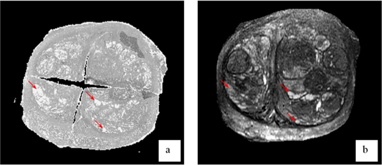
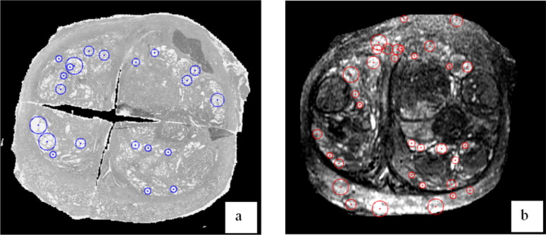
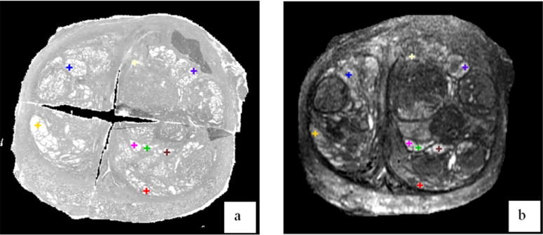
In our study toward the early diagnosis of prostate cancer, we proposed a computer-aided biopsy system, which aims to increase the diagnosis accuracy of prostate biopsy using population-based statistical information ( ) as well as patient-specific image information. As shown in Fig 1 , our proposed biopsy system consists of three modules, respectively for image-based biopsy optimization, atlas-based biopsy optimization, and integration and application of optimized biopsy strategies. In the atlas-based biopsy optimization module, biopsy needles are deployed at the locations where the statistical atlas of prostate cancer distribution exhibits higher cancer incidence. In the image-based biopsy optimization module, biopsy needles are deployed at the locations where the tissue appearances are similar to those of cancerous tissue. To achieve this objective, an automatic image analysis method is expected for labeling the suspicious cancerous tissue by learning the MR signatures of cancerous tissue from a sufficient number of prostate MR image samples where ground-truth cancer has been identified. However, since the ground-truth cancer information is only available in the histological images, it is necessary to warp the confirmed cancerous regions in histological images to MR images, in order to collect ground-truth cancer information in MR images. Figure 2 shows an example of warping a ground-truth cancerous region from the histological image to the MR image of the same prostate. The dark pink region in Fig 2 a indicates ground-truth cancerous region in the histological image, and the green region in Fig 2 c denotes the warped ground-truth cancerous region in the MR image.

Open full size image

Figure 1

Schematic description of our proposed computer-aided biopsy system. (1) Generate optimal biopsy strategy based on patient-specific image information. (2) Generate optimal biopsy strategy based on population-based statistical information. (3) Integrate the two biopsy strategies and apply them to an individual patient.

Open full size image

Figure 2

An example of warping a ground-truth cancerous region from the histological image to the magnetic resonance (MR) image of the same prostate. (a) Prostate histologic image, where the dark pink region denotes ground-truth cancer labeled by a pathologist. (b) Prostate T2-weighted MR image. (c) Prostate T2-weighted MR image with manually warped cancer ground truth as indicated by a green region.

Get Radiology Tree app to read full this article<

Methods

Get Radiology Tree app to read full this article<

Boundary Landmarks

Boundary landmarks detection

Get Radiology Tree app to read full this article<

Similarity definition of boundary landmarks

Get Radiology Tree app to read full this article<

S(xi,yj)=1−∥∥F¯¯¯(xi)−F¯¯¯(yj)∥∥ S

(

)

−

‖

(

)

−

(

)

‖

Get Radiology Tree app to read full this article<

Internal Landmarks

Get Radiology Tree app to read full this article<

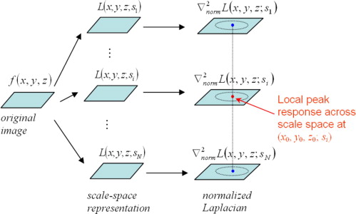
Salient structure detection with automatic scale selection

Get Radiology Tree app to read full this article<

L(x,y,z;s)=g(x,y,z;s)∗f(x,y,z) L

(

;

)

(

;

)

∗

(

)

where g(x,y,z;s)=1(2πs2)3/2e−(x2+y2+z2)/2s2 g

(

;

)

(

)

−

(

)

2 . Gaussian function is selected here as a convolution kernel, since it is stated as the unique kernel for generating a scale-space within the class of linear transformations ( ).

Get Radiology Tree app to read full this article<

∂ξ=s∂x ∂

∂

Get Radiology Tree app to read full this article<

∇normL(x,y,z;s)=∇ξL(x,y,z;s)=s∇L(x,y,z;s) ∇

(

;

)

∇

(

;

)

∇

(

;

)

Get Radiology Tree app to read full this article<

Internal landmarks detection

Get Radiology Tree app to read full this article<

f(x,y,z)=A(32s20)3/2e−((x−x0)2+(y−y0)2+(z−z0)2)/2(32s20) f

(

)

(

)

−

(

−

)

(

−

)

(

−

)

(

)

Get Radiology Tree app to read full this article<

L(x,y,z;s)=A(32s20+s2)3/2e−((x−x0)2+(y−y0)2+(z−z0)2)/2(32s20+s2) L

(

;

)

(

)

−

(

−

)

(

−

)

(

−

)

(

)

Get Radiology Tree app to read full this article<

Q(s)=max(x,y,z)∣∣(∇2normL(x,y,z;s)∣∣=∣∣(∇2normL(x0,y0,z0;s)∣∣=3As2(32s20+s2)5/2 Q

(

)

max

⁡

(

)

(

∇

(

;

)

(

∇

(

;

)

(

)

Get Radiology Tree app to read full this article<

dQds=9As(s20−s2)(32s20+s2)7/2 d

(

−

)

(

)

Because Eq 8 equals to zero when s = s 0 , the normalized Laplacian achieves its maximum at ( x 0 , y 0 , z 0 ; s 0 ) in the scale-space, which indicates a blob detected with center ( x 0 , y 0 , z 0 ) and size 32−−√s0 3

0 . In other words, if we detect a peak at a location ( x 0 , y 0 , z 0 ) with scale s 0 , it indicates that there might exist a blob centered at ( x 0 , y 0 , z 0 ) with the size of 32−−√s0 3

0 .

Get Radiology Tree app to read full this article<

Similarity definition of internal landmarks

Get Radiology Tree app to read full this article<

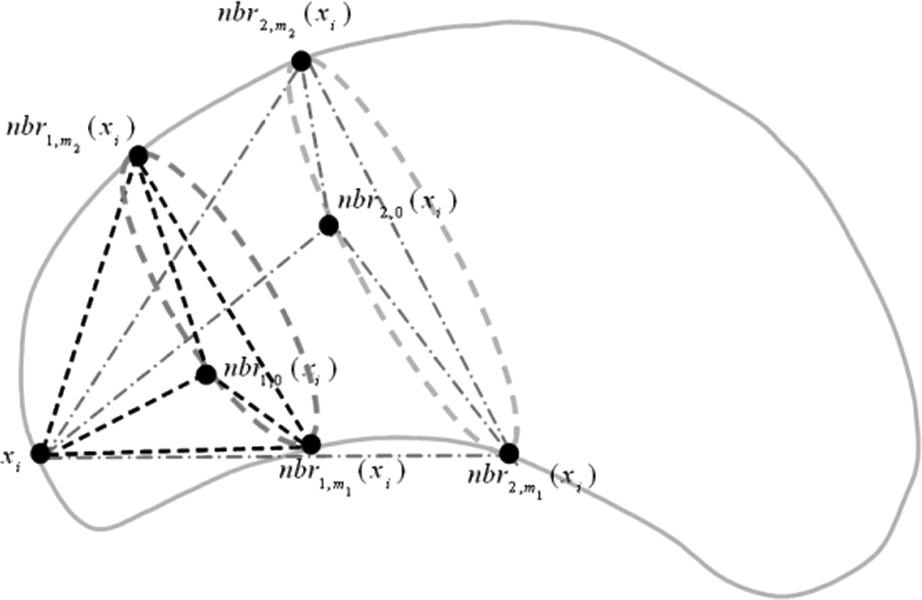
M(u,v)=max−α≤Δ≤α∑Ni=1NMI{V(u,i⋅su),T(V(v,i⋅sv);susv,Δ)} M

(

)

max

⁡

−

≤

∑

{

(

⋅

)

(

⋅

)

;

)

}

Where V ( u, R ) denotes a spherical local patch around the landmark u with the radius R . T(V; s, Δ θ ) is the transformation operator with a scaling factor s and a rotation factor Δ θ . The variable i is the size factor of the local patch where NMI is calculated, and N is the total number of multiple local patches used. NMI { · , · } denotes the normalized mutual information between two same-sized spherical volume images. (Δθ = π/8 π

8 and N = 3 in this study)

Get Radiology Tree app to read full this article<

Overall Similarity Function

Get Radiology Tree app to read full this article<

A={aik} A

{

}

Get Radiology Tree app to read full this article<

{∑I+1i=1aik=1(k=1,⋯,K);∑K+1k=1aik=1(i=1,⋯,I);aik∈[0,1]} {

∑

(

⋯

)

;

∑

(

⋯

)

;

∈

[

]

}

and

B={bjl} B

{

}

subject to

{∑J+1j=1bjl=1(l=1,⋯,L);∑L+1l=1bjl=1(j=1,⋯,J);bjl∈[0,1]} {

∑

(

⋯

)

;

∑

(

⋯

)

;

∈

[



]

}

It is worth noting that a ik and b jl have real values between 0 and 1, which denote the fuzzy correspondences between landmarks ( ). Also, an extra row (i.e., { a ( I +1) k } or { b ( J +1) 1 }) and an extra column (i.e., { a ( K +1) } or { b__j(L +1) 1 }) are added to each correspondence matrix (i.e., A or B ) for handling the outliers. If a landmark cannot find its correspondence, it is regarded as an outlier and the extra entry of this landmark will be set as 1.

Get Radiology Tree app to read full this article<

maxA,B,hE(A,B,h)=maxA,B,h{[α∑Ii=1∑Kk=1aikS(xi,yk)+β∑Jj=1∑Ll=1bjlM(uj,vl)]−λ[∑Ii=1∑Kk=1aikD(xi,h(yk))+∑Jj=1∑Ll=1bjlD(uj,h(vl))+∥W(h)∥2]−[τ(∑Ii=1∑Kk=1aiklogaik+∑Jj=1∑Ll=1bjllogbjl)−ζ(∑Ii=1∑Kk=1aik+∑Jj=1∑Ll=1bjl)]} max

⁡

(

)

max

⁡

{

[

∑

(

)

∑

(

)

]

−

[

∑

(

)

∑

(

)

‖

(

)

‖

]

−

[

(

∑

log

⁡

∑

log

⁡

)

−

(

∑

)

]

}

Here, matrixes A and B are the fuzzy correspondences matrixes subject to Eq 10 and 11 , and h denotes the transformation between histologic and MR images. The two terms in the first square bracket denote the similarity between landmarks, where S ( · , · ) and M ( · , · ) are the similarity between boundary landmarks and the similarity between internal landmarks, as defined in Eq 1 and 9 , respectively. The three terms in the second square bracket jointly place smoothness constraints on the transformation h . D ( · , · ) denotes the Euclidean distance between two points, and ‖ W ( h )‖ 2 is a smoothness measurement of h . In our study, because thin plate spline is selected to model the transformation h , the smoothing term is the “bending energy” of the transformation h , for example:

∥W(h)∥2=∫∫∫[(∂2h∂x2)2+(∂2h∂y2)2+(∂2h∂z2)2+2(∂2h∂x∂y)2+2(∂2h∂x∂z)2+2(∂2h∂y∂z)2]dxdydz ‖

(

)

‖

∫

[

(

∂

)

(

∂

)

(

∂

)

(

∂

)

(

∂

)

(

∂

)

]

The four terms in the third square bracket are used to direct the correspondences matrixes A and B converging to binary ( ). With a higher τ , the correspondences are forced to be more fuzzy and become a factor in “convexifying” the objective function. Although τ is gradually reduced to zero, the fuzzy correspondences become binary ( ).

Get Radiology Tree app to read full this article<

Results

Get Radiology Tree app to read full this article<

Data Preparation

Get Radiology Tree app to read full this article<

Experiments to Register Anatomic Structures of Prostates

Get Radiology Tree app to read full this article<

Table 1

Average Distances Between the Prostate Capsule Surfaces in Magnetic Resonance Images and in Warped Histologic Images

Method 1 (mm) Method 2 (mm) Method 3 (mm) Subject 1 0.92 0.66 0.62 Subject 2 1.02 0.78 0.83 Subject 3 0.97 0.61 0.61 Subject 4 0.95 0.65 0.63 Subject 5 1.03 0.70 0.72 Mean 0.98 0.68 0.68

Method 1: mutual information based affine registration method. Method 2: method using only boundary landmarks. Method 3: the proposed method.

Table 2

Volume Overlay Error Between the Prostate Glands in Magnetic Resonance Images and in Warped Histologic Images

Method 1 Method 2 Method 3 Subject 1 8.6% 5.8% 5.1% Subject 2 9.3% 6.8% 7.2% Subject 3 7.5% 5.3% 5.3% Subject 4 8.1% 5.0% 5.3% Subject 5 9.3% 7.0% 7.7% Mean 8.6% 6.0% 6.1%

Method 1: mutual information based affine registration method. Method 2: method using only boundary landmarks. Method 3: the proposed method.

Get Radiology Tree app to read full this article<

Table 3

Average Distances Between Manually and Automatically Labeled Corresponding Landmarks

Method 1 (mm) Method 2 (mm) Method 3 (mm) Subject 1 1.31 1.03 0.77 Subject 2 1.81 1.05 0.97 Subject 3 1.25 0.97 0.76 Subject 4 1.43 1.09 0.81 Subject 5 1.53 1.03 0.87 Mean 1.47 1.03 0.82

Method 1: mutual information based affine registration method. Method 2: method using only boundary landmarks. Method 3: the proposed method.

Get Radiology Tree app to read full this article<

Experiments to Warp Ground-Truth Cancerous Region

Get Radiology Tree app to read full this article<

Table 4

Volume Overlay Percentage Between Manually and Automatically Labeled Cancerous Regions

Method 1 Method 2 Method 3 Maximum 82.9% 87.5% 88.3% Minimum 55.9% 60.4% 64.1% Average 71.6% 75.5% 79.1%

Method 1: mutual information based affine registration method. Method 2: method using only boundary landmarks. Method 3: the proposed method.

Get Radiology Tree app to read full this article<

Conclusions

Get Radiology Tree app to read full this article<

References

1. Christens-Barry W.A., Partin A.W.: Quantitative grading of tissue and nuclei in prostate cancer for prognosis prediction. Johns Hopkins Apl Technical Digest 1997; 18: pp. 226-233.
2. Rifkin M., Zerhouni E., Gatsonis C., et. al.: Comparison of magnetic resonance imaging and ultrasonography in staging early prostate cancer. N Engl J Med 1990; 323: pp. 621-626.
3. Ikonen S., Kaerkkaeinen P., Kivisaari L., et. al.: Magnetic resonance imaging of clinically localized prostatic cancer. J Urol 1998; 159: pp. 915-919.
4. Madabhushi A., Feldman M., Metaxas D.N., et. al.: A novel stochastic combination of 3D texture features for automated segmentation of prostatic adenocarcinoma from high resolution MRI.2003. Presented at MICCAI.
5. Chan I., Wells W., Mulkern R.V., et. al.: Detection of prostate cancer by integration of line-scan diffusion, T2-mapping and T2-weighted magnetic resonance imaging; a multichannel statistical classifier. Med Phys 2003; 30: pp. 2390-2398.
6. Zhan Y., Shen D., Zeng J., et. al.: Targeted prostate biopsy using statistical image analysis. IEEE Trans Med Imaging 2007; 26: pp. 779-788.
7. Madabhushi A., Feldman M.D., Metaxas D.N., et. al.: Automated detection of prostatic adenocarcinoma from high-resolution ex vivo MRI. IEEE Trans Med Imaging 2005; 24: pp. 1611-1625.
8. Fix A., Stitzel S., Ridder G., et. al.: MK-801 neurotoxicity in cupric silver-stained sections: Lesion reconstruction by 3-dimensional computer image analysis. Toxicol Pathol 2000; pp. 84-90.
9. Moskalik A., Rubin M., Wojno K.: Analysis of three-dimensional Doppler ultrasonographic quantitative measures for the discrimination of prostate cancer. J Ultrasound Med 2001; 20: pp. 713-722.
10. Chui H., Rangarajan A.: A new point matching algorithm for non-rigid registration. Comp Vision Image Understanding 2003; 89: pp. 114-141.
11. Thompson P.M., Mega M.S., Woods R.P., et. al.: Cortical change in Alzheimer’s disease detected with a disease-specific population-based brain atlas. Cerebr Cortex 2001; 11: pp. 1-16.
12. Shen D.: 4D image warping for measurement of longitudinal brain changes.2004. Presented at Proceedings of the IEEE International Symposium on Biomedical Imaging, Arlington, VA.
13. Fan Y., Shen D., Davatzikos C.: Classification of structural images via high-dimensional image warping, robust feature extraction, and SVM.2005. Presented at MICCAI, Palm Springs, CA.
14. Rouet J.-M., Jacq J.-J., Roux C.: Genetic algorithms for a robust 3-D MR-CT registration. IEEE Trans Inform Technol Biomed 2000; 4: pp. 126-136.
15. Hill D.L.G., Hawkes D.G., Gleeson M.J., et. al.: Accurate frameless registration of MR and CT images of the head: applications in planning surgery and radiation therapy. Radiology 1994; 191: pp. 447-454.
16. Maes F., Collignon A., Vandermeulen D., et. al.: Multimodality image registration by maximization of mutual information. IEEE Trans Med Imaging 1997; 16: pp. 187-198.
17. Collignon A., Vandermeulen D., Suetens P., et. al.: 3D multimodality medical image registration using feature space clustering.Ayache N.1995.Springer-VerlagBerlin, Germany:pp. 195-204.
18. Wachowiak M.P.S., Zheng R., Zurada Y., et. al.: An approach to multimodal biomedical image registration utilizing particle swarm optimization. IEEE Trans Evol Comp 2004; 8: pp. 289-301.
19. Taylor L., Porter B., Nadasdy G., et. al.: Three-dimensional registration of prostate images from histology and ultrasound. Ultrasound Med Biol 2004; 30: pp. 161-168.
20. Jacobs M., Windham J., Soltanian-Zadeh H., et. al.: Registration and warping of magnetic resonance images to histological sections. Med Phys 1999; 26: pp. 1568-1578.
21. Schormann T., Zilles K.: Three-dimensional linear and nonlinear transformations: An integration of light microscopical and MRI data. Human Brain Map 1998; 6: pp. 339-347.
22. d’Aische AdB., Craene M.D., Geets X., et. al.: Efficient multi-modal dense field non-rigid registration: alignment of histological and section images. Med Image Anal 2004; 9: pp. 538-546.
23. Bardinet E., Ourselin S., Dormont D., et. al.: Co-registration of histological, optical and MR data of the human brain.2002. Presented at Medical Image Computing and Computer-Assisted Intervention, Tokyo, Japan.
24. Andronache A., Cattin P., Szekely G.: Adaptive subdivision for hierarchical non-rigid registration of multi-modal images using mutual information.2005. Presented at MICCAI.
25. Lorensen W.E., Cline H.E.: Marching cubes: a high resolution 3D surface reconstruction algorithm. Comp Graphics 1987; 21: pp. 163-169.
26. Shen D., Herskovits E.H., Davatzikos C.: An adaptive-focus statistical shape model for segmentation and shape modeling of 3D brain structures. IEEE Trans Med Imaging 2001; 20: pp. 257-270.
27. Witkin A.: Scale-space filtering: a new approach to multi-scale description.1984. Presented at IEEE International Conference on Acoustics, Speech, and Signal Processing, West Germany.
28. Lindeberg T.: Feature detection with automatic scale selection. Int J Comp Vis 1998; 30: pp. 77-116.
29. Lindeberg T.: Scale-space for discrete signals. IEEE Trans Pattern Anal Machine Intell 1990; 12: pp. 234-254.
30. Pauwels E.J.V.G., Fiddelaers L.J., Moons P., et. al.: An extended class of scale-invariant and recursive scale space filters. IEEE Trans Pattern Anal Machine Intell 1995; 17: pp. 691-701.
31. Lindeberg T.: Scale-space theory: a basic tool for analysing structures at different scales. J Appl Stat 1994; 21: pp. 223-261.
32. Studholme C.H., Hawkes D.L.G.: An overlap invariant entropy measure of 3D medical image alignment. Patt Recogn 1999; 32: pp. 71-86.
33. Hardy R.: Theory and applications of the multiquadric-biharmonic method. Comp Math Application 1990; 19: pp. 163-208.
34. Bookstein F.L.: Principal warps: thin-plate splines and the decomposition of deformations. IEEE Trans Pattern Anal Machine Intell 1989; 11: pp. 567-585.
35. Arad N., Reisfeld D.: Image warping using few anchor points and radial functions. Comp Graphics Forum 1995; 14: pp. 35-46.
36. Davatzikos C., Abraham F., Biros G., et. al.: Correspondence detection in diffusion tensor images.2006. Presented at ISBI, Washington, DC.
37. Xie Z., Farin G.E.: Image registration using hierarchical B-splines. IEEE Trans Visual Comp Graphics 2004; 10: pp. 85-94.
38. Rueckert D., Sonoda L.I., Hayes C., et. al.: Non-rigid registration using free-form deformations: application to breast MR images. IEEE Trans Med Imaging 1999; 18: pp. 712-721.
39. Yang J., Blum R.S., Williams J.P., et. al.: Non-rigid Image registration using geometric features and local salient region features.2006. Presented at IEEE Computer Society Conference on Computer Vision and Pattern Recognition, New York, NY.
40. Jenkinson M., Bannister P.R., Brady J.M., et. al.: Improved optimisation for the robust and accurate linear registration and motion correction of brain images. NeuroImage 2002; 17: pp. 825-841.
41. Zhan Y., Shen D.: Deformable segmentation of 3D ultrasound prostate images using statistical texture matching method. IEEE Trans Med Imaging 2006; 25: pp. 256-272.

Registering Histologic and MR Images of Prostate for Image-based Cancer Detection

Rationale and Objectives

Material and Methods

Results

Conclusions

Related work

Methods

Boundary Landmarks

Boundary landmarks detection

Similarity definition of boundary landmarks

Internal Landmarks

Salient structure detection with automatic scale selection

Internal landmarks detection

Similarity definition of internal landmarks

Overall Similarity Function

Results

Data Preparation

Experiments to Register Anatomic Structures of Prostates

Experiments to Warp Ground-Truth Cancerous Region

Conclusions

References

Further Reading

Abstracts of Funded National Institutes of Health Grants

Academic Technology Transfer and Radiology

Advances in Radiologic Image Analysis From MICCAI 2006