
Rationale and Objectives
The creation of two-dimensional (2D) ultrasound mosaics is becoming a common clinical practice with a high clinical value. The next step coming along with the increasing availability of 2D array transducers is the creation of three-dimensional mosaics. The correct alignment of multiple ultrasound images is, however, a complex task. In the literature of ultrasound registration, the alignment of two images has been often addressed, but not the alignment of multiple images. Therefore, we propose registration strategies for multiple image alignment and ultrasound specific similarity measures, which are able to cope with problems when aligning ultrasound images.
Materials and Methods
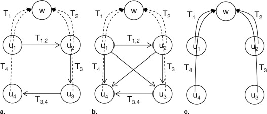
In this study, we investigate the following strategies for multiple image alignment: pairwise registration with a successive Lie group normalization and simultaneous registration, which urges the usage of multivariate similarity measures. We propose alternative multivariate extensions for similarity measures based on a maximum likelihood framework. Moreover, we take the inherent contamination of ultrasound images by speckle patterns into consideration by using alternative noise models based on multiplicative Rayleigh distributed noise. This leads us to ultrasound-specific similarity measures.
Results
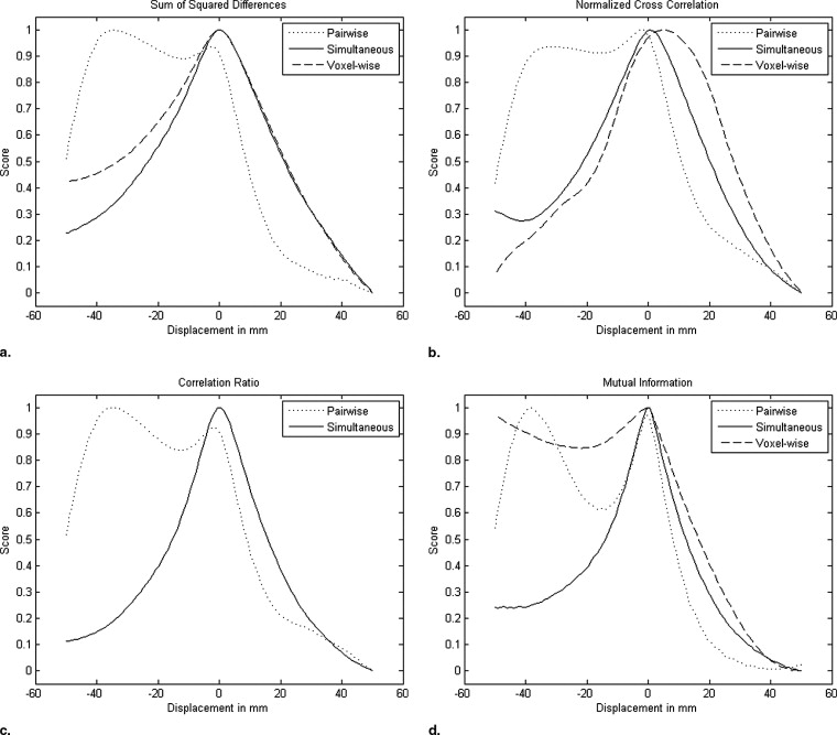
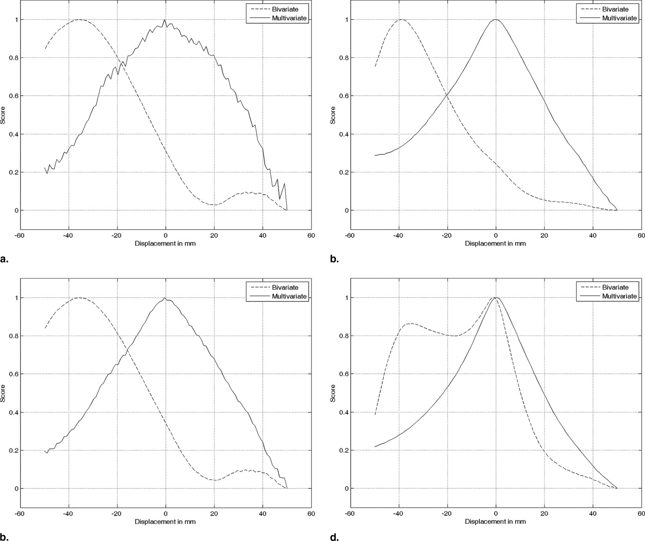
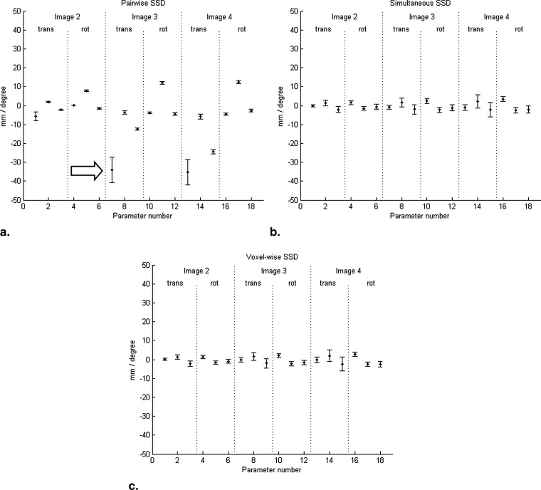
We compare the performances of pairwise and simultaneous registration approaches for the mosaicing scenario. Bivariate similarity measures are highly overlap-dependent, so that they rather favor the total overlap of the images than their correct alignment. Using ultrasound-specific bivariate measures leads to better results; however, a local optimum at the total overlap remains. In contrast, the derived multivariate similarity measures have a clear and single optimum at the correct alignment of the volumes.
Conclusion
The experiments indicate that standard, pairwise registration techniques have problems by aligning multiple ultrasound images with partial overlap. We demonstrate that the usage of an ultrasound specific similarity measure leads to better results for pairwise registration. The highest robustness, however, can be achieved by using simultaneous registration with the developed multivariate similarity measures.
At the moment, a paradigm shift is taking place in ultrasound (US) imaging, moving from two-dimensional (2D) to three-dimensional (3D) image acquisition. The next generation of 2D array US transducers with capacitive micromachined US transducer technology could accelerate this shift by offering superior and efficient volumetric imaging at a lower cost.
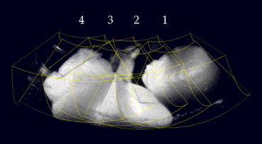
From a current perspective, the only drawbacks that remain are the limited field of view of the acquired images and the reflectance of the beam from structures with high acoustic impedance causing occlusion. The idea of mosaicing addresses these issues by combining the information of several images taken from different poses. The focus can rest on quality improvement by imaging the same scene from different directions, or the extension of the field of view by stitching together consecutively taken images. Whatever we are interested in, the first step is to calculate the correct global alignment, for which we propose solutions in this report.
Get Radiology Tree app to read full this article<
Clinical value of US mosaicing
Get Radiology Tree app to read full this article<
Get Radiology Tree app to read full this article<
Get Radiology Tree app to read full this article<
Problems Statement
Get Radiology Tree app to read full this article<
Get Radiology Tree app to read full this article<
Mosaicing Strategies
Get Radiology Tree app to read full this article<
Get Radiology Tree app to read full this article<
Pairwise Registration with Lie Normalization
Get Radiology Tree app to read full this article<
Get Radiology Tree app to read full this article<
τi,j=T−1i⋅Tj⋅Ti,j. τ
i
,
j
=
T
i
−
1
·
T
j
·
T
i
,
j
.
Get Radiology Tree app to read full this article<
Get Radiology Tree app to read full this article<
μ2τ(τi,j)=logId(τi,j)T⋅∑−1ττ⋅logId(τi,j). μ
τ
2
(
τ
i
,
j
)
=
log
Id
(
τ
i
,
j
)
T
⋅
∑
τ
τ
−
1
⋅
log
Id
(
τ
i
,
j
)
.
Get Radiology Tree app to read full this article<
Get Radiology Tree app to read full this article<
[Tˆ1,…,Tˆn]=argmin[T1,…,Tn]12∑(i,j)ωi,j⋅μ2τ(τi,j). [
T
1
,
…
,
T
n
]
=
arg
min
[
T
1
,
…
,
T
n
]
1
2
∑
(
i
,
j
)
ω
i
,
j
·
μ
τ
2
(
τ
i
,
j
)
.
with the quality weights ω i,j . These weights model the quality of each pairwise registration. Because we are interested in an automated registration, we use the amount of overlap as an indicator of the registration quality. The final algorithm using the Lie group normalization is stated in Table 1 . The registration is accepted if the total error τt=∑(i,j)ωi,j⋅μ2τ(τi,j) τ
t
=
∑
(
i
,
j
)
ω
i
,
j
·
μ
τ
2
(
τ
i
,
j
) is below a scenario dependent threshold δ. An alternative for using an acceptance criterion based on the absolute error τ t would be to calculate the relative error between two iterations τitert−τiter−1t τ
t
iter
−
τ
t
iter
−
1 .
Table 1
Algorithm for Pairwise Registration with Lie Group Normalization
1. Start with initial global transformations T = {T 1 , … , T n } 2. Do 2.1 Deduce initial pairwise transformations T i,j from T T using T i,j = T j −1 ·T i 2.2 Compute all pairwise registrations T i,j with intensity-based rigid registration 2.3 Estimate new T from calculated T i,j with Lie group normalization in Equation 3 3. While (τ t > δ) 4. Return T T
Get Radiology Tree app to read full this article<
Simultaneous Registration
Get Radiology Tree app to read full this article<
Get Radiology Tree app to read full this article<
Get Radiology Tree app to read full this article<
Table 2
Algorithm for Semi-simultaneous Registration
1. For number of cycles 1.1 For each i in {1, … , n } 1.1.1 Simultaneously register image u__i to { u__1 , … , u__i–1 , u__i+1 , … u__n } for k optimization steps, changing matrix T__i 1.2 END 2. END 3. Return T
Get Radiology Tree app to read full this article<
Get Radiology Tree app to read full this article<
Multivariate Similarity Measures
Get Radiology Tree app to read full this article<
logL(T,ε,f)=logP(u|v,T,ε,f)=logP(ε=u(x)−f(v(T(x)))) log
L
(
T
,
ε
,
f
)
=
log
P
(
u
|
v
,
T
,
ε
,
f
)
=
log
P
(
ε
=
u
(
x
)
−
f
(
v
(
T
(
x
)
)
)
)
with P the probability density function. In the work of Viola ( ) and Roche et al ( ), the deduction of the four measures based on this equation is shown by varying the assumptions for the intensity mapping. We are extending this approach to multiple images under the assumption of conditional independent images. The extended MLE denoting the transformed images u↓i=ui(Ti(⋅)) u
i
↓
=
u
i
(
T
i
(
·
)
)
logL(T,ε→,f→)=logP(u↓1u↓2,…,u↓n,ε→,f→) log
L
(
T
,
ε
→
,
f
→
)
=
log
P
(
u
1
↓
u
2
↓
,
…
,
u
n
↓
,
ε
→
,
f
→
)
=logP(ε2=u↓1−f2(u↓2),…,εn=u↓1−fn(u↓n))
log
P
(
ε
2
=
u
1
↓
−
f
2
(
u
2
↓
)
,
…
,
ε
n
=
u
1
↓
−
f
n
(
u
n
↓
)
)
=∑ni=2logP(εi=u↓1−fi(u↓i))
∑
i
=
2
n
log
P
(
ε
i
=
u
1
↓
−
f
i
(
u
i
↓
)
)
with intensity mappings f→=(f2,…,fn) f
→
=
(
f
2
,
…
,
f
n
) and Gaussian noise ε→=(ε2,…,εn) ε
→
=
(
ε
2
,
…
,
ε
n
) . Each summand corresponds to the bivariate formula in Equation 4 , and the deduction of the four similarity measures can therefore be done analogously, as elsewhere ( ). This shows that we directly obtain multivariate extensions of that form by summing up the bivariate measures. In this type of extension, we pick one reference image, in the formulas above u 1 , which works well for the semi-simultaneous registration approach. Setting up a similarity matrix M with the entries M__i,j = SM ( u__i__, u__j ), this corresponds to summing up its first row. An adaptation of this approach to the full-simultaneous registration is obtained by summing up the whole similarity matrix, which can often be limited to the upper triangular part because of the symmetry of the measures. Additionally, the pairs are weighted by an overlap-dependent factor ω i,j emphasizing pairs with high overlap. The final similarity measures are shown in Table 3 .
Table 3
Summary of Bivariate and Multivariate Similarity Measures in Shortened Notation
Pairwise Semi-simultaneous Full-simultaneous Voxel-wise Sum of squared differencesE[(u−v↓)2] E
[
(
u
−
v
↓
)
2
] ∑ni=2ω1,iE[(u1−u↓i)2] ∑
i
=
2
n
ω
1
,
i
E
[
(
u
1
−
u
i
↓
)
2
] ∑i<jωi,jE[(u↓i−u↓j)2] ∑
i
<
j
ω
i
,
j
E
[
(
u
i
↓
−
u
j
↓
)
2
] ∑xk∈ΩωkEi[(μk−u↓i(xk))2] ∑
x
k
∈
Ω
ω
k
E
i
[
(
μ
k
−
u
i
↓
(
x
k
)
)
2
] Normalized cross-correlationE[u˜1⋅v˜↓] E
[
u
˜
1
⋅
v
˜
↓
] ∑ni=2ω1,iE[u˜1⋅u˜↓i] ∑
i
=
2
n
ω
1
,
i
E
[
u
˜
1
⋅
u
˜
i
↓
] ∑i<jωi,jE[u˜↓1⋅u˜↓j] ∑
i
<
j
ω
i
,
j
E
[
u
˜
1
↓
⋅
u
˜
j
↓
] ∑xk∈ΩωkE[u˜↓1⋅u˜↓2…u˜↓3] ∑
x
k
∈
Ω
ω
k
E
[
u
˜
1
↓
⋅
u
˜
2
↓
…
u
˜
3
↓
] Correlation-ratioVar[E(u∣∣v↓)]Var(u) Var
[
E
(
u
|
v
↓
)
]
Var
(
u
) ∑ni=2ω1,iVar[E(u1∣∣u↓i)]Var(u1) ∑
i
=
2
n
ω
1
,
i
Var
[
E
(
u
1
|
u
i
↓
)
]
Var
(
u
1
) ∑i≠jωi,jVar[E(u↓i∣∣uj)]Var(u↓i) ∑
i
≠
j
ω
i
,
j
Var
[
E
(
u
i
↓
|
u
j
)
]
Var
(
u
i
↓
) — Mutual information (MI) MI( u , v ↓ )∑ni=2ωi,jMI(ui,u↓i) ∑
i
=
2
n
ω
i
,
j
MI
(
u
i
,
u
i
↓
) ∑i<jωi,jMI(u↓i,u↓j) ∑
i
<
j
ω
i
,
j
M
I
(
u
i
↓
,
u
j
↓
) ∑xk∈ΩωkH(Pk) ∑
x
k
∈
Ω
ω
k
H
(
P
k
)
Get Radiology Tree app to read full this article<
Get Radiology Tree app to read full this article<
logL(T)=logP(u↓1,u↓2,…,u↓n) log
L
(
T
)
=
log
P
(
u
1
↓
,
u
2
↓
,
…
,
u
n
↓
)
=1|Ω|log∏xk∈ΩPk(u↓1(xk),…,u↓n(xk))
1
|
Ω
|
log
∏
x
k
∈
Ω
P
k
(
u
1
↓
(
x
k
)
,
…
,
u
n
↓
(
x
k
)
)
≈1|Ω|∑xk∈Ωlog∏ni=1Pk(u↓i(xk)) ≈
1
|
Ω
|
∑
x
k
∈
Ω
log
∏
i
=
1
n
P
k
(
u
i
↓
(
x
k
)
)
with the grid Ω. By further assuming a Gaussian distribution of values at each location with mean μ__k and variance σ2k σ
k
2 , the log-likelihood function is
logL⎛⎝⎜T⎞⎠⎟=1|Ω|∑xk∈Ω∑ni=1log⎛⎝⎜12π√σe−12(u↓i(xk)−μk)2σ2k⎞⎠⎟ log
L
(
T
)
=
1
|
Ω
|
∑
x
k
∈
Ω
∑
i
=
1
n
log
(
1
2
π
σ
e
−
1
2
(
u
i
↓
(
x
k
)
−
μ
k
)
2
σ
k
2
)
≈−1|Ω|∑xk∈Ω1σ2k∑ni=1(u↓i(xk)−μk)2⋅ ≈
−
1
|
Ω
|
∑
x
k
∈
Ω
1
σ
k
2
∑
i
=
1
n
(
u
i
↓
(
x
k
)
−
μ
k
)
2
·
We consider this criterion as a voxel-wise extension of SSD because similar assumptions for its pairwise deduction shown elsewhere ( ) hae been used. When not taking the assumption of a Gaussian distribution, Equation 6 can be further developed as was done for the congealing by Zollei et al ( ):
logL(T)=1N∑xk∈Ω∑ni=1logPk(u↓i(xk)) log
L
(
T
)
=
1
N
∑
x
k
∈
Ω
∑
i
=
1
n
log
P
k
(
u
i
↓
(
x
k
)
)
≈∑xk∈ΩH(Pk) ≈
∑
x
k
∈
Ω
H
(
P
k
)
with the sample entropy H. We added the congealing criterion ( ) as an extension of MI to Table 3 , because they are both based on the estimation of the entropy H, although they have different properties. We also use a voxel-wise criterion for NCC that, in our opinion, captures the basic idea of it by multiplying the values at each voxel location of the normalized images u˜i u
˜
i . This is obviously not a rigorous deduction, but rather based on analogies. For all, we added the weighting factor ω k emphasizing locations with a higher number of overlapping images. The usual extensions based on higher dimensional probability density functions are not applicable to mosaicing because they are not flexible enough to allow for varying numbers of overlapping images.
Get Radiology Tree app to read full this article<
US-specific Similarity Measures
Get Radiology Tree app to read full this article<
Get Radiology Tree app to read full this article<
SK 1 : Multiplicative Rayleigh Noise
Get Radiology Tree app to read full this article<
u(x)=v(T(x))⋅ε u
(
x
)
=
v
(
T
(
x
)
)
·
ε
with the Rayleigh distribution
P(y)=π⋅y2⋅exp(−π⋅y24),y>0 P
(
y
)
=
π
·
y
2
·
exp
(
−
π
·
y
2
4
)
,
y
0
having the variance 2π 2
π . Setting it into the MLE framework, Equation 4 , leads to:
logL(T,ε)=log∏xk⊂Ω1v(T(xk))P(u(xk)v(T(xk))) log
L
(
T
,
ε
)
=
log
∏
x
k
⊂
Ω
1
v
(
T
(
x
k
)
)
P
(
u
(
x
k
)
v
(
T
(
x
k
)
)
)
≈∑xk∈Ωlog(u(xk)v(T(xk))2)−π4u(xk)2v(T(xk))2 ≈
∑
x
k
∈
Ω
log
(
u
(
x
k
)
v
(
T
(
x
k
)
)
2
)
−
π
4
u
(
x
k
)
2
v
(
T
(
x
k
)
)
2
Get Radiology Tree app to read full this article<
SK 2 : Signal-dependent Gaussian Noise
Get Radiology Tree app to read full this article<
u(x)=v(T(x))+v(T(x))−−−−−−√⋅ε⋅ u
(
x
)
=
v
(
T
(
x
)
)
+
v
(
T
(
x
)
)
·
ε
·
Get Radiology Tree app to read full this article<
Get Radiology Tree app to read full this article<
logL(T,ε)=log∏xk∈Ω1v(T(xk))√exp(−[u(xk)−v(T(xk))]22⋅σ2⋅v(T(xk)) log
L
(
T
,
ε
)
=
log
∏
x
k
∈
Ω
1
v
(
T
(
x
k
)
)
exp
(
−
[
u
(
x
k
)
−
v
(
T
(
x
k
)
)
]
2
2
·
σ
2
·
v
(
T
(
x
k
)
)
=∑xk∈Ω−log[v(T(xk))]−[u(xk)−v(T(xk))]22⋅σ2⋅v(T(xk))
∑
x
k
∈
Ω
−
log
[
v
(
T
(
x
k
)
)
]
−
[
u
(
x
k
)
−
v
(
T
(
x
k
)
)
]
2
2
⋅
σ
2
·
v
(
T
(
x
k
)
)
Get Radiology Tree app to read full this article<
CD 1 : Division of Rayleigh Noises
Get Radiology Tree app to read full this article<
u(x)=v(T(x))⋅εwithε=ε1ε2 u
(
x
)
=
v
(
T
(
x
)
)
·
ε
with
ε
=
ε
1
ε
2
and the probability density function for a division of Rayleigh noises is:
P(y)=2⋅y(y2+1)2,y>0. P
(
y
)
=
2
⋅
y
(
y
2
+
1
)
2
,
y
0.
Get Radiology Tree app to read full this article<
Get Radiology Tree app to read full this article<
logL(T,ε)=log∏xk∈Ω1v(T(xk))P(u(xk)v(T(xk))) logL
(
T
,
ε
)
=
log
∏
x
k
∈
Ω
1
v
(
T
(
x
k
)
)
P
(
u
(
x
k
)
v
(
T
(
x
k
)
)
)
=log∏xk∈Ω1v(T(xk))2⋅u(xk)v(T(xk))((u(xk)v(T(xk)))2+1)2
log
∏
x
k
∈
Ω
1
v
(
T
(
x
k
)
)
2
⋅
u
(
x
k
)
v
(
T
(
x
k
)
)
(
(
u
(
x
k
)
v
(
T
(
x
k
)
)
)
2
+
1
)
2
=∑xk∈Ωlog2⋅u(xk)v(T(xk))2−2⋅log[(u(xk)v(T(xk)))2+1]
∑
x
k
∈
Ω
log
2
⋅
u
(
x
k
)
v
(
T
(
x
k
)
)
2
−
2
⋅
log
[
(
u
(
x
k
)
v
(
T
(
x
k
)
)
)
2
+
1
]
≈∑xk∈Ωlogu(xk)−logv(T(xk))−log[(u(xk)v(T(xk)))2+1]. ≈
∑
x
k
∈
Ω
log
u
(
x
k
)
−
log
v
(
T
(
x
k
)
)
−
log
[
(
u
(
x
k
)
v
(
T
(
x
k
)
)
)
2
+
1
]
.
Get Radiology Tree app to read full this article<
CD 2 : Logarithm of Division of Rayleigh Noises
Get Radiology Tree app to read full this article<
logu(x)=log[v(T(x))⋅ε] log
u
(
x
)
=
log
[
v
(
T
(
x
)
)
·
ε
]
=logv(T(x))+logε.
log
v
(
T
(
x
)
)
+
log
ε
.
Get Radiology Tree app to read full this article<
Get Radiology Tree app to read full this article<
ε(x)=exp(u˜(x)+v˜(x)) ε
(
x
)
=
exp
(
u
˜
(
x
)
+
v
˜
(
x
)
)
leading to the log-likelihood function:
logL(T,ε)=log∏xk∈Ωexp(u˜(xk))exp(v˜(xk))⋅P(exp(u˜(xk)−u˜(xk))) log
L
(
T
,
ε
)
=
log
∏
x
k
∈
Ω
exp
(
u
˜
(
x
k
)
)
exp
(
v
˜
(
x
k
)
)
⋅
P
(
exp
(
u
˜
(
x
k
)
−
u
˜
(
x
k
)
)
)
=log∏xk∈Ωexp(u˜(xk))exp(v˜(xk))⋅2⋅exp(u˜(xk)−u˜(xk))[exp(u˜(xk)−u˜(xk))2+1]2
log
∏
x
k
∈
Ω
exp
(
u
˜
(
x
k
)
)
exp
(
v
˜
(
x
k
)
)
·
2
⋅
exp
(
u
˜
(
x
k
)
−
u
˜
(
x
k
)
)
[
exp
(
u
˜
(
x
k
)
−
u
˜
(
x
k
)
)
2
+
1
]
2
=log∏xk∈Ω2⋅exp(2(u˜(xk)−u˜(xk)))[exp(2(u˜(xk)−u˜(xk)))+1]2
log
∏
x
k
∈
Ω
2
⋅
exp
(
2
(
u
˜
(
x
k
)
−
u
˜
(
x
k
)
)
)
[
exp
(
2
(
u
˜
(
x
k
)
−
u
˜
(
x
k
)
)
)
+
1
]
2
≈∑xk∈Ωu˜(xk)−v˜(xk)−log[exp(2(u˜(xk)−v˜(xk)))+1]. ≈
∑
x
k
∈
Ω
u
˜
(
x
k
)
−
v
˜
(
x
k
)
−
log
[
exp
(
2
(
u
˜
(
x
k
)
−
v
˜
(
x
k
)
)
)
+
1
]
.
Get Radiology Tree app to read full this article<
Multivariate Extension
Get Radiology Tree app to read full this article<
Table 4
Summary of Multivariate Ultrasound-specific Similarity Measures
SK 1 SK 2 ∑i≠jωi,j⋅E[log(uiu2j)−π4u2iu2j] ∑
i
≠
j
ω
i
,
j
⋅
E
[
log
(
u
i
u
j
2
)
−
π
4
u
i
2
u
j
2
] ∑i≠jωi,j⋅E[loguj+(ui−uj)2uj] ∑
i
≠
j
ω
i
,
j
⋅
E
[
log
u
j
+
(
u
i
−
u
j
)
2
u
j
] CD 1 CD 2 ∑i≠jωi,j⋅E[loguiu2j((uiuj)2+1)−2] ∑
i
≠
j
ω
i
,
j
⋅
E
[
log
u
i
u
j
2
(
(
u
i
u
j
)
2
+
1
)
−
2
] ∑i≠jωi,j⋅E[u˜i−u˜j−log(e2(u˜i−u˜j)+1)] ∑
i
≠
j
ω
i
,
j
⋅
E
[
u
˜
i
−
u
˜
j
−
log
(
e
2
(
u
˜
i
−
u
˜
j
)
+
1
)
]
Get Radiology Tree app to read full this article<
Results
Get Radiology Tree app to read full this article<
Get Radiology Tree app to read full this article<

Get Radiology Tree app to read full this article<
Get Radiology Tree app to read full this article<
Get Radiology Tree app to read full this article<
Get Radiology Tree app to read full this article<
Get Radiology Tree app to read full this article<
Get Radiology Tree app to read full this article<
Get Radiology Tree app to read full this article<
Conclusion
Get Radiology Tree app to read full this article<
Get Radiology Tree app to read full this article<
Get Radiology Tree app to read full this article<
Get Radiology Tree app to read full this article<
Get Radiology Tree app to read full this article<
References
1. Wang Z., Slabaugh G., Unal G., et. al.: Registration of ultrasound images using an information-theoretic feature detector. 4th IEEE International Symposium 2007; pp. 736-739.
2. Kim S.H., Choi B.I., Kim K.W., et. al.: Extended field-of-view sonography: advantages in abdominal applications. J Ultrasound Med 2003; 22: pp. 385-394.
3. Peetrons P.: Ultrasound of muscles. Eur Radiol 2002; 12: pp. 35-43.
4. Leung Y., Roshier A., Johnson S., et. al.: Demonstration of the appearance of the paraspinal musculoligamentous structures of the cervical spine using ultrasound. Clin Anat 2005; 18: pp. 96-103.
5. Ying M., Sin M.H.: Comparison of extended field of view and dual image ultrasound techniques: accuracy and reliability of distance measurements in phantom study. Ultrasound Med Biol 2005; 31: pp. 79-83.
6. Dietrich C., Ignee A., Gebel M., et. al.: Imaging of the abdomen. Z Gastroenterol 2002; 40: pp. 965-970.
7. Henrich W., Schmider A., Kjos S., et. al.: Advantages of and applications for extended field-of-view ultrasound in obstetrics. Arch Gynecol Obstet 2003; V268: pp. 121-127.
8. Kuhl H., Schreckenberg M., Rulands D., et. al.: High-resolution transthoracic real-time three-dimensional echocardiography quantitation of cardiac volumes and function using semi-automatic border detection and comparison with cardiac magnetic resonance imaging. J Am Coll Cardiol 2004; 43: pp. 2083-2090.
9. Jenkins C., Bricknell K., Hanekom L., et. al.: Reproducibility and accuracy of echocardiographic measurements of left ventricular parameters using real-time three-dimensional echocardiography. J Am Coll Cardiol 2004; 44: pp. 878-886.
10. Gee A.H., Treece G.M., Prager R.W., et. al.: Rapid registration for wide field-of-view freehand 3D ultrasound. IEEE Trans Med Imaging 2003; 22: pp. 1344-1357.
11. Poon T., Rohling R.: Three-dimensional extended field-of-view ultrasound. Ultrasound Med Biol 2005; 32: pp. 357-369.
12. O’Donnell M., Skovoroda R.: Internal displacement and strain imaging using ultrasonic speckle tracking. IEEE Trans Ultrason Ferroelect Freq Control 1994; 41: pp. 3.
13. Penney G.P., Blackall J.M., Hamady M.S., et. al.: Registration of freehand 3D ultrasound and magnetic resonance liver images. Med Image Anal 2004; 8: pp. 81-91.
14. Abd-Elmoniem K., Youssef A., Kadah Y.: Real-time speckle reduction and coherence enhancement in ultrasoundimaging via nonlinear anisotropic diffusion. Biomed Engin IEEE Trans 2002; 49: pp. 997-1014.
15. Kotropoulos C., Magnisalis X., Pitas I., et. al.: Nonlinear ultrasonic image processing based on signal-adaptive filters and self-organizing neural networks. Image Proc IEEE Trans 1994; 3: pp. 65-77.
16. Pennec X. Statistical computing on manifolds for computational anatomy (Thesis). Habilitation a diriger des recherches, Universite Nice Sophia-Antipolis (Dec. 2006).
17. Vercauteren T., Perchant A., Malandain G., et. al.: Robust mosaicing with correction of motion distortions and tissue deformation for in vivo fibered microscopy. Med Image Anal 2006; 10: pp. 673-692.
18. Zollei L., Learned-Miller E., Grimson E.W.W.: Efficient population registration of 3D data. ICCV 2005; pp. 291-301.
19. Benjemaa R., Schmitt F.: Fast global registration of 3D sampled surfaces using a multi-buffer technique. Image Vision Comp 1999; 17: pp. 113-123.
20. Viola P.A.: Alignment by maximization of mutual information.1995.PhD thesis, Massachusetts Institute of Technology
21. Roche A., Malandain G., Ayache N.: Unifying maximum likelihood approaches in medical image registration. Int J Imaging Syst Tech Special Issue 3D Imaging 2000; 11: pp. 71-80.
22. Strintzis M., Kokkinidis I.: Maximum likelihood motion estimation in ultrasound image sequences. Signal Proc Lett IEEE 1997; 4: pp. 156-157.
23. Cohen B., Dinstein I.: New maximum likelihood motion estimation schemes for noisy ultrasound images. Pattern Recognition 2002; 35: pp. 455-463.
24. Boukerroui D., Noble J., Brady M.: Velocity estimation in ultrasound images: a block matching approach. Inf Process Med Imaging 2003; 18: pp. 586-598.
25. Revell J., Mirmehdi M., McNally D.: Combined ultrasound speckle pattern similarity measures. BMVA Press 2004; pp. 149-153.
26. Papoulis A., Pillai U.S.: Probability, random variables and stochastic processes.2001.McGraw-HillNew York
27. Press W., Teukolsky S., Vetterling W., et. al.: Numerical recipes in C: the art of scientific computing.2002.Cambridge University Press
28. Soler P., Delso G., Villain N., et. al.: Superresolution spatial compounding techniques with application to 3D breast ultrasound imaging. SPIE Med Imaging 2006: Ultrasonic Imaging and Signal Processing 2006; 6147: pp. 281-292.
29. Wachinger C., Shams R., Navab N.: Estimation of acoustic impedance from multiple ultrasound images with application to spatial compounding.2008. IEEE Computer Society Workshop on Mathematical Methods in Biomedical Image Analysis, Anchorage, AK, June 27–28.