Reliable and Computationally Efficient Maximum-Likelihood Estimation of “Proper” Binormal ROC Curves

Rationale and Objectives

Estimation of ROC curves and their associated indices from experimental data can be problematic, especially in multireader, multicase (MRMC) observer studies. Wilcoxon estimates of area under the curve (AUC) can be strongly biased with categorical data, whereas the conventional binormal ROC curve-fitting model may produce unrealistic fits. The “proper” binormal model (PBM) was introduced by Metz and Pan to provide acceptable fits for both sturdy and problematic datasets, but other investigators found that its first software implementation was numerically unstable in some situations. Therefore, we created an entirely new algorithm to implement the PBM.

Materials and Methods

This paper describes in detail the new PBM curve-fitting algorithm, which was designed to perform successfully in all problematic situations encountered previously. Extensive testing was conducted also on a broad variety of simulated and real datasets. Windows, Linux, and Apple Macintosh OS X versions of the algorithm are available online at http://xray.bsd.uchicago.edu/krl/ .

Results

Plots of fitted curves as well as summaries of AUC estimates and their standard errors are reported. The new algorithm never failed to converge and produced good fits for all of the several million datasets on which it was tested. For all but the most problematic datasets, the algorithm also produced very good estimates of AUC standard error. The AUC estimates compared well with Wilcoxon estimates for continuously distributed data and are expected to be superior for categorical data.

Conclusion

This implementation of the PBM is reliable in a wide variety of ROC curve-fitting tasks.

Radiological research often lies at the interface between human observers (radiologists) and technology. When technologies are applied to a population of patients, they usually produce extremely variable information (e.g., because both small and large lesions are represented), and in clinical settings this variable information is interpreted by human observers with different training, experience and capabilities. Such observers sometimes produce different final decisions when evaluating the same information; moreover, a single radiologist may report different results when reading a particular image on multiple occasions. Therefore, overall assessments of radiological technology often must deal with large variability, the modeling of which is complex ( ), so multireader, multicase (MRMC) methodologies are used increasingly to evaluate new diagnostic techniques ( ).

MRMC and some simpler statistical analyses require estimation of a population figure of merit or index such as area under the ROC curve (AUC) for a subset of the data, conditional upon one or more covariates; in MRMC analysis one needs to estimate AUC, for example, for each imaging-modality/reader combination. Maximum-likelihood estimation (MLE) often is used to calculate these indices from a given dataset because of its good statistical properties and clear interpretation ( ). MLE of ROC curves from categorical confidence-rating data was first used by Dorfmann and Alf ( ), who described a procedure based on the conventional binormal model (CvBM).

Get Radiology Tree app to read full this article<

Materials and methods

Get Radiology Tree app to read full this article<

Data Categorization Scheme

Get Radiology Tree app to read full this article<

Initial Estimates

Get Radiology Tree app to read full this article<

Optimization

Get Radiology Tree app to read full this article<

Standard-Error Estimation

Get Radiology Tree app to read full this article<

Evaluation Studies

Get Radiology Tree app to read full this article<

Results

Get Radiology Tree app to read full this article<

Real Data

Get Radiology Tree app to read full this article<

Continuously Distributed Simulation Data

Get Radiology Tree app to read full this article<

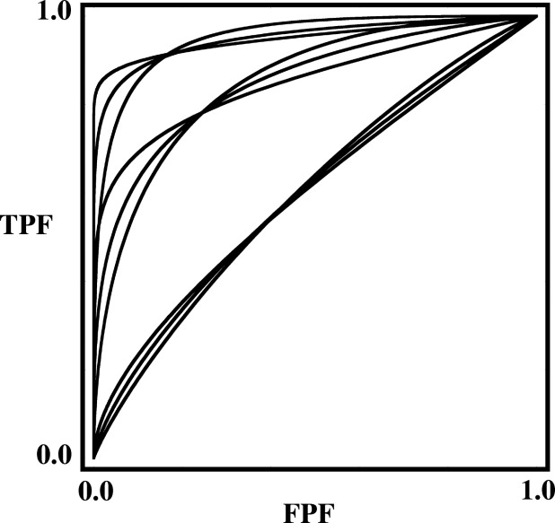
Table 1

AUC and Parameter Values of the Population ROC Curves Used in the Simulation Studies

AUC Value Curve Shape (skew) High Medium Symmetrical_d a__c__d a__c__d a__c_ 0.60000 0.100000 −0.154357 0.358000 −0.046907 0.358287 0.0 0.85000 1.24365 −0.428571 1.46571 −0.140000 1.46574 0.0 0.95000 0.0999998 −0.853738 2.32400 −0.292369 2.32618 0.0

The corresponding plots are shown in Figure 4 . These AUC values and curve shapes bracket the ranges encountered in most medical-imaging studies. The parameter values are specified to six significant digits because this precision is required for accurate calculation of some AUC values.

Get Radiology Tree app to read full this article<

Table 2

Results of the Simulations for AUC = 0.60000

ROC Curve Shape (skew) No. of Actually Positive or Negative Cases 25 50 75 100 200 300 Symmetric (no skew)AUC¯¯¯¯¯¯¯¯ A

¯ 0.618 0.608 0.604 0.603 0.6003 0.600SE 0.070 0.051 0.042 0.038 0.027 0.023SEˆ¯¯¯¯¯ S

¯ 0.071 0.052 0.043 0.038 0.027 0.022SE/SE w 0.73 0.81 0.85 0.89 0.94 0.96 Medium skewAUC¯¯¯¯¯¯¯¯ A

¯ 0.621 0.610 0.606 0.604 0.602 0.600SE 0.069 0.050 0.041 0.036 0.026 0.022SEˆ¯¯¯¯¯ S

¯ 0.070 0.051 0.042 0.037 0.026 0.022SE/SE w 0.85 0.89 0.90 0.92 0.94 0.95 High skewAUC¯¯¯¯¯¯¯¯ A

¯ 0.627 0.617 0.613 0.612 0.608 0.606SE 0.068 0.049 0.040 0.034 0.024 0.020SEˆ¯¯¯¯¯ S

¯ 0.069 0.050 0.041 0.035 0.025 0.020SE/SE w 0.84 0.87 0.86 0.87 0.86 0.86

The value shown at the top of each column represents the number of actually positive or negative cases (i.e., half of the total number of cases) used in each simulated experiment. The rows within each curve-shape block indicate: AUC¯¯¯¯¯¯¯¯ A

¯ , average of the estimated AUC value; SE , empirical standard deviation of the estimated AUC values; SEˆ¯¯¯¯¯ S

¯ , average of the estimated standard errors determined from the individual AUC estimates; SE/SE w , ratio of the empirical standard deviation of the MLE AUC estimates to that of the Wilcoxon AUC estimates. Each table entry was obtained from 20,000 datasets to reduce uncertainties to less than three digits (except for the SE ratios, which have two-digit precision), so no confidence intervals are shown. The largest bias/standard-deviation ratios (0.27 for the symmetric curve, 0.40 for the highly skewed curve) were observed for the datasets composed of 25 actually negative and 25 actually positive cases. The estimated ratio of MLE to Wilcoxon standard error carries an uncertainty of approximately ±1%; this precision is related to the number of datasets, rather than to the size of each dataset, so it is approximately the same for all numbers of cases.

Table 3

Results of the Simulations for AUC = 0.85000

ROC Curve Shape (skew) No. of Actually Positive or Negative Cases 25 50 75 100 200 300 400 500 Symmetric (no skew)AUC¯¯¯¯¯¯¯¯ A

¯ 0.855 0.852 0.851 0.851 0.851 0.8505 0.8503 0.8503SE 0.053 0.038 0.031 0.026 0.018 0.015 0.013 0.012SEˆ¯¯¯¯¯ S

¯ 0.052 0.037 0.030 0.026 0.018 0.015 0.013 0.012SE/SE w 0.98 1.00 0.99 1.00 0.99 0.99 1.00 1.00 Medium skewAUC¯¯¯¯¯¯¯¯ A

¯ 0.855 0.852 0.851 0.8506 0.8504 0.8502 0.8502 0.8502SE 0.052 0.038 0.031 0.027 0.019 0.016 0.013 0.012SEˆ¯¯¯¯¯ S

¯ 0.051 0.037 0.031 0.027 0.019 0.015 0.013 0.012SE/SE w 0.95 0.99 0.99 1.00 1.00 1.00 0.99 0.98 High skewAUC¯¯¯¯¯¯¯¯ A

¯ 0.867 0.860 0.857 0.856 0.853 0.852 0.8516SE 0.047 0.034 0.028 0.024 0.017 0.014 0.012SEˆ¯¯¯¯¯ S

¯ 0.046 0.033 0.027 0.024 0.017 0.014 0.012SE/SE w 0.84 0.86 0.86 0.86 0.88 0.89 0.88

The notation used here is defined in the caption of Table 2 . For the smallest datasets (25 actually negative and 25 actually positive cases), the ratio of bias to standard deviation is 0.01 for the worst symmetrical population ROC and 0.36 for the worst highly skewed ROC. Again, the ratio of MLE to Wilcoxon standard error has an uncertainty of approximately ±1%.

Table 4

Results of the Simulations for AUC = 0.95000

ROC Curve Shape (skew) No. of Actually Positive or Negative Cases 25 50 75 100 200 300 Symmetric (no skew)AUC¯¯¯¯¯¯¯¯ A

¯ 0.951 0.951 0.9505 0.9504 0.9503 0.9501SE 0.028 0.019 0.016 0.014 0.010 0.008SEˆ¯¯¯¯¯ S

¯ 0.029 0.020 0.016 0.014 0.010 0.008SE/SE w 0.96 0.95 0.95 0.95 0.95 0.95 Medium skewAUC¯¯¯¯¯¯¯¯ A

¯ 0.954 0.951 0.9503 0.9501 0.9500 0.9500SE 0.028 0.021 0.018 0.015 0.011 0.009SEˆ¯¯¯¯¯ S

¯ 0.028 0.021 0.017 0.015 0.011 0.009SE/SE w 0.96 0.95 0.95 0.95 0.95 0.95 High skewAUC¯¯¯¯¯¯¯¯ A

¯ 0.961 0.957 0.956 0.955 0.953 0.952SE 0.025 0.018 0.015 0.013 0.009 0.008SEˆ¯¯¯¯¯ S

¯ 0.024 0.018 0.015 0.013 0.009 0.008SE/SE w 0.96 0.96 0.96 0.96 0.95 0.95

The notation used here is defined in the caption of Table 2 . For the smallest datasets, the ratio of bias to standard deviation is 0.035 for the worst symmetrical population ROC and 0.44 for the worst highly skewed ROC. As in Tables 2 and 3 , the estimated ratio of MLE to Wilcoxon standard error has an uncertainty of approximately ±1%.

Get Radiology Tree app to read full this article<

Discussion

Get Radiology Tree app to read full this article<

References

1. Roe C.A., Metz C.E.: Variance-component modeling in the analysis of receiver operating characteristic index estimates. Acad Radiol 1997; 4: pp. 587-600.
2. Dorfman D.D., Berbaum K.S., Metz C.E.: Receiver operating characteristic rating analysis. Invest Radiol 1992; 27: pp. 723-731.
3. Obuchowski N.A., Rockette H.E.: Hypothesis-testing of diagnostic-accuracy for multiple readers and multiple tests—An ANOVA approach with dependent observations. Commun Stat Simulation Comput 1995; 24: pp. 285-308.
4. Beiden S.V., Wagner R.F., Campbell G.: Components-of-variance models and multiple-bootstrap experiments: An alternative method for random-effects, receiver operating characteristic analysis. Acad Radiol 2000; 7: pp. 341-349.
5. Wagner R.F., Beiden S.V., Campbell G., Metz C.E., Sacks W.M.: Assessment of medical imaging and computer-assist systems: Lessons from recent experience. Acad Radiol 2002; 9: pp. 1264-1277.
6. Toledano A.Y., Gatsonis C.: Ordinal regression methodology for ROC curves derived from correlated data. Stat Med 1996; 15: pp. 1807-1826.
7. Gallas B.D.: One-shot estimate of MRMC variance: AUC. Acad Radiol 2006; 13: pp. 353-362.
8. Dorfman D.D., Alf E.: Maximum-likelihood estimation of parameters of signal-detection theory and determination of confidence intervals—Rating-method data. J Math Psychol 1969; 6: pp. 487-496.
9. Hanley J.A.: Receiver operating characteristic (ROC) methodology: The state of the art. Crit Rev Diagn Imaging 1989; 29: pp. 307-335.
10. Swets J.A.: Form of empirical ROCs in discrimination and diagnostic tasks: Implications for theory and measurement of performance. Psychol Bull 1986; 99: pp. 181-198.
11. Metz C.E., Herman B.A., Shen J.H.: Maximum likelihood estimation of receiver operating characteristic (ROC) curves from continuously distributed data. Stat Med 1998; 17: pp. 1033-1053.
12. Metz C.E.: Some practical issues of experimental design and data analysis in radiological ROC studies. Invest Radiol 1989; 24: pp. 234-245.
13. Hanley J.A.: The robustness of the “binormal” assumptions used in fitting ROC curves. Med Decis Making 1988; 8: pp. 197-203.
14. Obuchowski N.A., Beiden S.V., Berbaum K.S., et. al.: Multireader, multicase receiver operating characteristic analysis: An empirical comparison of five methods. Acad Radiol 2004; 11: pp. 980-995.
15. Metz C.E., Pan X.: “Proper” binormal ROC curves: Theory and maximum-likelihood estimation. J Math Psychol 1999; 43: pp. 1-33.
16. Pan X., Metz C.E.: The “proper” binormal model: Parametric receiver operating characteristic curve estimation with degenerate data. Acad Radiol 1997; 4: pp. 380-389.
17. Dorfman D.D., Berbaum K.S.: A contaminated binormal model for ROC data: Part III. Acad Radiol 2000; 7: pp. 438-447.
18. Bandos A.I., Rockette H.E., Gur D.: Incorporating utility-weights when comparing two diagnostic systems: A preliminary assessment. Acad Radiol 2005; 12: pp. 1293-1300.
19. Obuchowski N.A.: Estimating and comparing diagnostic tests’ accuracy when the gold standard is not binary. Acad Radiol 2005; 12: pp. 1198-1204.
20. Edwards D.C., Metz C.E., Kupinski M.A.: Ideal observers and optimal ROC hypersurfaces in N-class classification. IEEE Trans Med Imaging 2004; 23: pp. 891-895.
21. Metz C.E.: ROC methodology in radiologic imaging. Invest Radiol 1986; 21: pp. 720-733.
22. Flannery B.P., Teukolsky S.A., Press W.H., Vetterling W.T.: 1992.Cambridge University PressCambridge, England/New York
23. Gay D.M.: Subroutines for unconstrained minimization using a model trust-region approach. ACM Trans Math Software 1983; 9: pp. 503-524.
24. DeLong E.R., DeLong D.M., Clarke-Pearson D.L.: Comparing the areas under two or more correlated receiver operating characteristic curves: A nonparametric approach. Biometrics 1988; 44: pp. 837-845.
25. Efron B., Tibshirani R.: 1993.Chapman & HallNew York
26. Rao C.R.: 1965.WileyNew York
27. Papoulis A.: 1984.McGraw-HillNew York
28. Campbell S.L., Meyer C.D.: 1991.Dover PublicationsNew York
29. Rao C.R., Mitra S.K.: 1971.WileyNew York
30. McClish D.K.: Analyzing a portion of the ROC curve. Med Decis Making 1989; 9: pp. 190-195.
31. Jiang Y., Metz C.E., Nishikawa R.M.: A receiver operating characteristic partial area index for highly sensitive diagnostic tests. Radiology 1996; 201: pp. 745-750.
32. Metz C., Kronman H.: Statistical significance tests for binormal ROC curves. J Math Psychol 1980; 22: pp. 218-243.
33. Kupinski M.A., Edwards D.C., Giger M.L., Metz C.E.: Ideal observer approximation using Bayesian classification neural networks. IEEE Trans Med Imaging 2001; 20: pp. 886-899.
34. Glantz S.A.: 2002.McGraw-Hill Medical Publishing DivisionNew York
35. Metz C.E.: Basic principles of ROC analysis. Semin Nucl Med 1978; 8: pp. 283-298.
36. Shiraishi J., Katsuragawa S., Ikezoe J., et. al.: Development of a digital image database for chest radiographs with and without a lung nodule: Receiver operating characteristic analysis of radiologists’ detection of pulmonary nodules. AJR Am J Roentgenol 2000; 174: pp. 71-74.
37. Bamber D.: Area above ordinal dominance graph and area below receiver operating characteristic graph. J Math Psychol 1975; 12: pp. 387-415.

Reliable and Computationally Efficient Maximum-Likelihood Estimation of “Proper” Binormal ROC Curves

Rationale and Objectives

Materials and Methods

Results

Conclusion

Materials and methods

Data Categorization Scheme

Numerical Issues With Functions Related to the Proper Binormal Model

Initial Estimates

Optimization

Standard-Error Estimation

Evaluation Studies

Results

Real Data

Continuously Distributed Simulation Data

Discussion

References

Further Reading

“Binary” and “Non-Binary” Detection Tasks Are Current Performance Measures Optimal?

2D or Not 2D That is the Question, But 3D is the Answer

3D and 2D Delayed-Enhancement Magnetic Resonance Imaging for Detection of Myocardial Infarction Preclinical and Clinical Results