Rationale and Objectives

The quantitative assessment of neck lymph nodes in the context of malignant tumors requires an efficient segmentation technique for lymph nodes in tomographic three-dimensional (3D) datasets. We present a stable 3D mass-spring model for lymph node segmentation in computed tomography (CT) datasets.

Materials and Methods

For the first time our model concurrently represents the characteristic gray value range, directed contour information, and shape knowledge, which leads to a robust and efficient segmentation process.

Results

Our model design and the segmentation accuracy were both evaluated with 40 lymph nodes from five clinical CT datasets containing malignant tumors of the neck.

Conclusion

The segmentation accuracy proved to be comparable to that of manual segmentations by experienced users and significantly reduced the time and interaction needed for the lymph node segmentation.

The assessment of lymph nodes plays an important role in the diagnosis, staging, treatment and therapy control of malignant tumors and their metastases. Currently magnetic resonance imaging and computed tomography (CT) scans of the respective regions allow for a three-dimensional (3D) assessment of the pathologic situation. For surgery and radiation planning, as well as for therapy control, an exact quantitative analysis of the lymph nodes’ volume, growth, and their infiltration of and distance to neighboring structures are essential. This demands a segmentation of the lymph nodes from the 3D datasets.

Lymph node segmentation often has to be performed manually by delineation of the contour in all involved slices of the 3D dataset. This may take up to 20 minutes per dataset, when many enlarged lymph nodes are contained ( ). This effort makes an accurate quantitative lymph node evaluation often unfeasible in the time-critical clinical routine. We present an efficient model-based segmentation technique for enlarged lymph nodes (1–3 cm) in CT datasets of the neck, which significantly reduces the time and interaction effort for lymph node segmentation.

Get Radiology Tree app to read full this article<

Open full size image

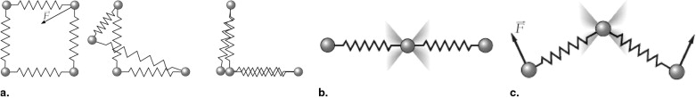
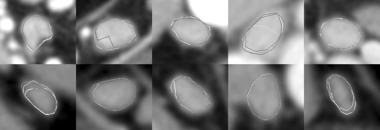
Figure 1

Different anatomic situations in computed tomography head and neck data: (a) isolated neck lymph node, (b) two adjacent lymph nodes, (c) neck lymph node adjacent to M. sternocleidomastoideus , (d) lymph node touching high-contrast structure (blood vessel), (e) lymph node with a central necrosis (dark).

Get Radiology Tree app to read full this article<

State of the art

Get Radiology Tree app to read full this article<

Materials and methods

Get Radiology Tree app to read full this article<

Stable 3D Mass-Spring Models

Get Radiology Tree app to read full this article<

Design of the Lymph Node Model

Get Radiology Tree app to read full this article<

Segmentation Process

Get Radiology Tree app to read full this article<

Step 1: Initial placement of the model in the dataset

Get Radiology Tree app to read full this article<

Step 2: Automatic determination of gray value range

Get Radiology Tree app to read full this article<

Table 1

Model Simulation Parameters (According to Previous Work) ( )

Parameter Category Parameter Description Symbol Value Model adaptation Simulation step size Δ t 0.02 Tolerance (stopping criterion) ε 0.01 mm Simulation steps (stopping criterion) n 5 Weighting of force components Torsion forces_ω t_ 25 Spring forces_ω f_ 20 Gradient sensor forces_ω sg_ 9 Intensity sensor forces_ω si_ 6 Constants for model elements Torsion constant_T ij_ 1 Spring stiffness (surface)S ij 0.01 Spring stiffness (functional unit)S ij 10 Mass_m i_ 1 Gray value range Lower interval margin_g min_ 150 HU Upper interval margin_g max_ 100 HU

Get Radiology Tree app to read full this article<

Step 3: Model adaptation

Get Radiology Tree app to read full this article<

Results and evaluation

Get Radiology Tree app to read full this article<

Table 2

Datasets Used for the Evaluation

Dataset Size Voxel Size Miscellaneous X/Y Z X/Y Z Slice thickness Contrast agent Device Lymph Nodes 1 512 65 0.28 3 3 mm Yes Siemens 26 2 512 61 0.28 3 3 mm Yes Siemens 5 3 512 26 0.41 1.95 2 mm No Siemens 10 4 512 61 0.45 3 3 mm No Siemens 10 5 512 42 0.44 5 5 mm Yes Siemens 6 6 512 63 0.42 3 3 mm Yes GE 15 7 512 262 0.47 0.7 1 mm Yes Philips 17 8 512 229 0.51 0.51 1 mm Yes Siemens 5 9 512 31 0.53 3 3 mm No Siemens 6 10 512 161 0.41 1.5 3 mm Yes Philips 35 11 512 52 0.35 3.9 4 mm Yes PI, Inc. 11

Get Radiology Tree app to read full this article<

Qualitative Evaluation of the Model Design

Get Radiology Tree app to read full this article<

Shape stability due to torsion forces

Get Radiology Tree app to read full this article<

Adaptation to lymph node size

Get Radiology Tree app to read full this article<

Functional unit of gradient and intensity sensors

Get Radiology Tree app to read full this article<

Quantitative Evaluation of Segmentation Accuracy

Get Radiology Tree app to read full this article<

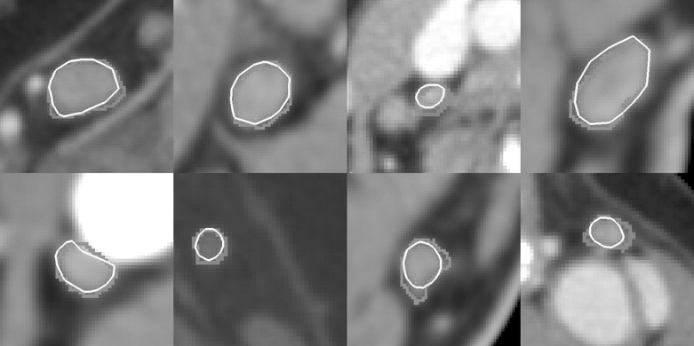
Table 3

Results of the Quantitative Evaluation

Dataset 1 2 3 4 5 Mean surface distance (mm) User A 0.420 0.353 0.401 0.311 0.296 User B 0.488 0.406 0.444 0.271 0.279 Model 0.421 0.309 0.596 0.583 0.416 Hausdorff distance (mm) User A 3.513 2.401 3.238 1.213 1.575 User B 4.113 2.644 3.225 1.150 1.725 Model 3.913 2.350 3.825 1.700 1.925 Volumetric segmentation error (%) User A 45.88 69.38 43.25 35.13 37.00 User B 45.63 65.25 50.88 29.88 33.13 Model 44.38 50.75 51.38 51.75 38.88

Get Radiology Tree app to read full this article<

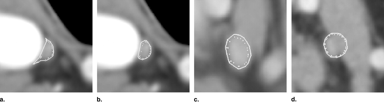
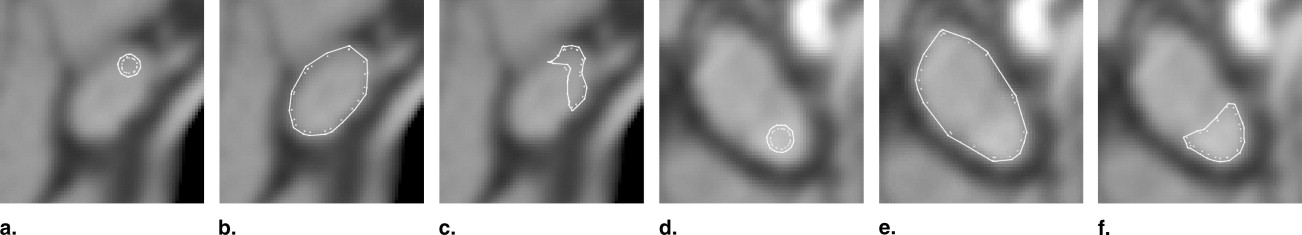
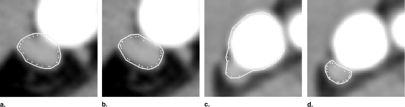
Robustness of the Method

Get Radiology Tree app to read full this article<

Conclusion

Get Radiology Tree app to read full this article<

References

1. Cordes J., Dornheim J., Preim B., et. al.: Strauss: Preoperative segmentation of neck CT datasets for the planning of neck dissections. Proc SPIE Med Imaging 2006: Image Processing 2006;
2. Rogowska J., Batchelder K., Gazelle G., et. al.: Evaluation of selected two-dimensional segmentation techniques for computed tomography quantification of lymph nodes. Investig Radiol 1996; 13: pp. 138-145.
3. Honea D.M., Ge Y., Snyder W.E., et. al.: Lymph node segmentation using active contours. Proc SPIE Med Imaging 1997: Image Processing 1997; 3034: pp. 265-273.
4. Honea D., Snyder W.E.: Three-dimensional active surface approach to lymph node segmentation. Proc SPIE Med Imaging 1999: Image Processing 1999; 3361: pp. 1003-1011.
5. Yan J., Zhuang T., Zhao B., et. al.: Lymph node segmentation from CT images using fast marching method. Comp Med Imaging Graphics 2004; 28: pp. 33-38.
6. Kuhnigk J.-M., Dicken V., Bornemann L., et. al.: Fast automated segmentation and reproducible volumetry of pulmonary metastases in CT-scans for therapy monitoring. MICCAI 2004; pp. 933-941.
7. Dornheim L., Tönnies K.D., Dornheim J.: Stable dynamic 3D shape models. Int Conf Image Proc (ICIP) 2005;
8. Dornheim L., Dornheim J., Tönnies K.D.: Automatic generation of dynamic 3D models for medical segmentation tasks. SPIE Med Imaging 2006;
9. Unal G., Slabaugh G., Ess A., et. al.: Semi-automatic lymph node segmentation in LN-MRI. Int Conf Image Proc (ICIP) 2006;
10. Cohen I., Cohen L.D., Ayache N.: Using deformable surfaces to segment 3d images and infer differential structures. CVGIP: Image Understanding 1992; 56: pp. 242-263.
11. Delingette H.: Adaptive and deformable models based on Simplex Meshes.IEEE Workshop of Non-Rigid and Articulated Objects.1994.
12. Montagnat J., Delingette H.: Volumetric medical images segmentation using shape-constrained deformable models.CVRMed.1997.pp. 13-22.

Segmentation of Neck Lymph Nodes in CT Datasets with Stable 3D Mass-Spring Models

Rationale and Objectives

Materials and Methods

Results

Conclusion

State of the art

Materials and methods

Stable 3D Mass-Spring Models

Design of the Lymph Node Model

Segmentation Process

Step 1: Initial placement of the model in the dataset

Step 2: Automatic determination of gray value range

Step 3: Model adaptation

Results and evaluation

Qualitative Evaluation of the Model Design

Shape stability due to torsion forces

Adaptation to lymph node size

Functional unit of gradient and intensity sensors

Quantitative Evaluation of Segmentation Accuracy

Robustness of the Method

Conclusion

References

Further Reading

Abstracts of Funded National Institutes of Health Grants

Academic Technology Transfer and Radiology

Advances in Radiologic Image Analysis From MICCAI 2006