Segmentation of the Bones in MRIs of the Knee Using Phase, Magnitude, and Shape Information

Rationale and Objectives

The segmentation of textured anatomy from magnetic resonance images (MRI) is a difficult problem. We present an approach that uses features extracted from the magnitude and phase of the MRI signal to segment the bones in the knee. Moreover, we show that by incorporating shape information, more accurate and anatomically valid segmentations are obtained.

Materials and Methods

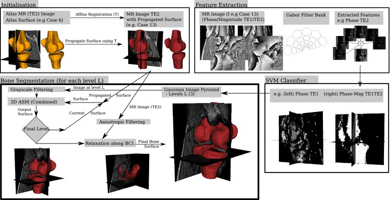
Eighteen volunteers were scanned in a whole-body 3T clinical scanner using a transmit-receive quadrature extremity coil. A gradient-echo sequence was used to acquire three-dimensional (3D) volumes of raw complex image data consisting of phase and magnitude information. These images were manually segmented and features were extracted using a bank of Gabor filters. The extracted features were then used to train a support vector machine (SVM) classifier. Each image was then automatically segmented using both the SVM classifier and a 3D active shape model (ASM) driven by the classifier.

Results

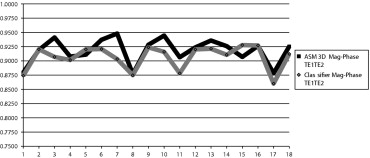
The use of phase and magnitude information from both echoes obtained the most accurate classifier results with an average dice similarity coefficient of 0.907. The use of 3D ASMs further improved the robustness, accuracy and anatomic validity of the segmentations with an overall DSC of 0.922 and an average point to surface error along the bone-cartilage interface of 0.73 mm.

Conclusions

Our results demonstrate that the incorporation of phase and multiple echoes improve the results obtained by the classifier. Moreover, we show that 3D ASMs provide a robust and accurate way of using the classifier to obtain anatomically valid segmentation results.

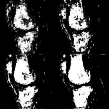
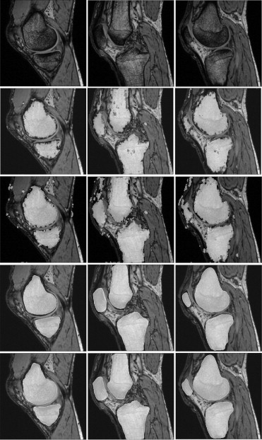
Magnetic resonance imaging (MRI) is a widely available and well accepted non invasive imaging technique. MRI acquisition is performed in k-space where a complex signal is acquired and reconstructed to produce a complex image, with phase and magnitude components as shown Fig 1 . The development of algorithms to allow the automatic and semiautomatic segmentation of MRIs has been the focus of much research. However, most of this research only uses the magnitude of the acquired complex MR signal, discarding the phase information.

Open full size image

Figure 1

Example sagittal slice (Case 11) showing the ( left ) phase and ( right ) magnitude at top T E1 = 4.9 milliseconds and bottom T E2 = 8.6 milliseconds.

Get Radiology Tree app to read full this article<

Materials and methods

MRI Acquisition

Get Radiology Tree app to read full this article<

Feature Extraction

Get Radiology Tree app to read full this article<

Iφ(x,y,z)=I(x,y,z)A(x,y,z)=ejφ(x,y,z). I

(

)

(

)

(

)

(

)

where A(x,y,z) A

(

) is the magnitude of the complex image. As a result, both the magnitude image A(x,y,z) A

(

) and the complex phase image Iφ(x,y,z) I

(

) can be Fourier transformed and filtered with the same bank of Gabor filters, producing 2 different sets of features.

Get Radiology Tree app to read full this article<

Classification

Get Radiology Tree app to read full this article<

3D ASM

Get Radiology Tree app to read full this article<

A 3D statistical shape model of the bones is used to represent the variability in shape of the bones. The approach used to automatically obtain the corresponding landmarks required, to build the SSM, was previously described elsewhere ( ) and follows the minimum description length optimization framework ( ). The number of training shapes in this model was increased using a bootstrap approach where the model was used to accurately segment the manual segmentations of the dual echo images (using an ASM and then a deformable model based relaxation). All the extracted surfaces were used in the model to create a combined SSM (consisting of the patella, tibia, and femur bones) that incorporated 42 different knees, each consisting of p j ; j = 1, 2, … , M (= 23,046) points.

Get Radiology Tree app to read full this article<

Segmentation System

Get Radiology Tree app to read full this article<

Validation Methodology

Get Radiology Tree app to read full this article<

Results

Get Radiology Tree app to read full this article<

Table 1

Mean (Standard Deviation) of the Dice Similarity Coefficient on the Bone Segmentation over the 14 Testing Datasets Segmented Three Times with Three Different Training Datasets ( CV 1 to CV 4 )

T E 1 T E 2 T E 1 T E 2 Support vector machine classifier Phase 0.68 (0.07) 0.73 (0.04) 0.83 (0.05) Magnitude 0.78 (0.05) 0.81 (0.04) 0.88 (0.03) Mag-phase 0.85 (0.03) 0.85 (0.02) 0.907 (0.021) ASM three-dimensional Mag-phase — — 0.918 (0.022) Relaxed Mag-phase — — 0.922 (0.021)

Get Radiology Tree app to read full this article<

Table 2

Mean (Standard Deviation) of the DSC on the Bone Segmentation over the Datasets

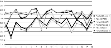
Patella Tibia Femur Affine_T E_ 2 0.60 (0.19) 0.82 (0.07) 0.83 (0.08) Three-dimensional active shape model Mag-phase_T E_ 1 T E 2 0.856 (0.028) 0.918 (0.030) 0.924 (0.028) Relaxed Mag-phase_T E_ 1 T E 2 0.870 (0.029) 0.920 (0.030) 0.929 (0.026)

Each segmented 51 times (three different training datasets [from CV 1 to CV 4 ] using 17 different atlas image initializations) except cases 17 and 18, which were segmented 68 times.

Get Radiology Tree app to read full this article<

Discussion

Get Radiology Tree app to read full this article<

Acknowledgment

Get Radiology Tree app to read full this article<

References

1. Haacke E., Xu Y.: The role of voxel aspect ratio in determining apparent vascular phase behavior in susceptibility weighted imaging. Magn Reson Med 2006; 24: pp. 155-160.
2. Graichen H., von Eisenhart-Rothe R., Vogl K.H., et. al.: Quantitative assessment of cartilage status in osteoarthritis by quantitative magnetic resonance imaging: technical validation for use in analysis of cartilage volume and further morphologic parameters. Arthritis Rheum 2004; 50: pp. 811-816.
3. Li K., Millington S., Wu X., et. al.: Simultaneous segmentation of multiple closed surfaces using optimal graph searching. Inform Proc Med Imaging 2005; 3565: pp. 406-417.
4. Tamez-Pena J.G., Barbu-McInnis M., Totterman S.: Knee cartilage extraction and bone-cartilage interface analysis from 3D MRI data sets. SPIE: Med Imaging 2004; 5370: pp. 1774-1784.
5. Lorigo L.M., Faugeras O., Grimson W.E.L., et. al.: Segmentation of bone in clinical knee MRI using texture-based geodesic active contours. MICCAI ’98 1998; 1496: pp. 1195-1204.
6. van Ginneken B., Frangi A.F., Staal J.J., et. al.: IEEE Trans Med Imaging 2002; 21: pp. 924-933. 2002
7. Haase A., Frahm J., Matthaei D., et. al.: Imaging: rapid NMR imaging using low flip-angle pulses. J Magnet Res 1986; 67: pp. 258-266.
8. Bovik A., Clark M., Geisler W.: Multichannel texture analysis using localized spatial filters. IEEE Trans Pattern Anal Machine Intell 1990; 12: pp. 55-73.
9. Grigorescu S.E., Petkov N., Kruizinga P.: Comparison of texture features based on Gabor filters. IEEE Trans Image Proc 2002; 11: pp. 1160-1167.
10. Bourgeat P., Fripp J., Janke A., et. al.: The use of unwrapped phase in MR image segmentation: a preliminary study. MICCAI’05 2005; 3750: pp. 813-820.
11. Bourgeat P., Fripp J., Stanwell P., Ramadan S., Ourselin S.: MR image segmentation of the knee bone using phase information. Med Image Anal 2007; 11: pp. 325-335.
12. Vapnik V.N.: The nature of statistical learning theory.1995.Springer VerlagNew York
13. Fan R.-E., Chen P.-H., Lin C.-J.: Working set selection using the second order information for training SVM. J Machine Learn Res 2005; 6: pp. 1889-1918.
14. Zhan Y., Shen D.: An adaptive error penalization method for training an efficient and generalized SVM. Patt Recog 2006; 39: pp. 342-350.
15. Cootes T.F., Taylor C.J., Cooper D.H., et. al.: Active shape models—their training and application. Comp Vis Image Understanding 1995; 61: pp. 38-59.
16. Keleman A., Szekeley H., Gerig G.: Three dimensional model-based segmentation of brain MRI. IEEE Trans Med Imaging 1999; 18: pp. 828-839.
17. Zhao Z., Aylward S.R., Teoh E.K.: A novel 3D partitioned active shape model for segmentation of brain MR images. LNCS 2005; 3749: pp. 221-228.
18. van Assen H.C., Danilouchkine M.G., Frangi A.F., et. al.: SPASM: a 3D-ASM for segmentation of sparse and arbitrarily oriented cardiac MRI data. Med Image Anal 2006; 10: pp. 286-303.
19. Zhan Y, Shen D. Automated segmentation of 3D US prostate images using statistical texture-based matching method. MICCAI’03 20003; 2878:688-696.
20. Fripp J., Crozier S., Warfield S.K., Ourselin S.: Automatic segmentation of the bone and extraction of the bone-cartilage interface from magnetic resonance images of the knee. Phys Med Biol 2007; 52: pp. 1617-1631.
21. Davies RhH., Twining C.J., Cootes T.F., et. al.: Statistical shape models using direct optimisation of description length. Proc 7th Euro Conf Computer Vis 2002; 2352: pp. 3-202.
22. Ourselin S., Roche A., Subsol G., et. al.: Reconstructing a 3D structure from serial histological sections. Image Vis Comp 2001; 19: pp. 2-31.
23. Vollmer J., Mencl R., Müller H.: Improved Laplacian smoothing of noisy surface meshes. Comp Graphics Forum 1999; 18: pp. 131-138.
24. Otsu N.: A threshold selection method from gray level histograms. IEEE Trans Sys Man Cybernet 1979; 9: pp. 62-66.
25. Dice L.R.: Measures of the amount of ecologic association between species. Ecology 1945; 26: pp. 297-302.

Segmentation of the Bones in MRIs of the Knee Using Phase, Magnitude, and Shape Information

Rationale and Objectives

Materials and Methods

Results

Conclusions

Materials and methods

MRI Acquisition

Feature Extraction

Classification

3D ASM

Segmentation System

Validation Methodology

Results

Discussion

Acknowledgment

References

Further Reading

3D Shape Analysis of the Supraspinatus Muscle

A Computer-Based Radiology Simulator as a Learning Tool to Help Prepare First-Year Residents for Being On Call

A Review of Research Into the Development of Radiologic Expertise Implications for Computer-Based Training