Semiautomatic Mammographic Parenchymal Patterns Classification Using Multiple Statistical Features

Rationale and Objectives

Our project was to investigate a complete methodology for the semiautomatic assessment of digital mammograms according to their density, an indicator known to be correlated to breast cancer risk. The BI-RADS four-grade density scale is usually employed by radiologists for reporting breast density, but it allows for a certain degree of subjective input, and an objective qualification of density has therefore often been reported hard to assess. The goal of this study was to design an objective technique for determining breast BI-RADS density.

Materials and Methods

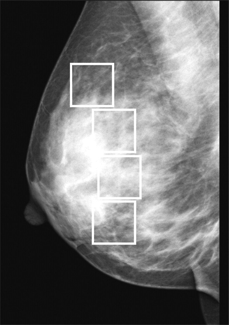
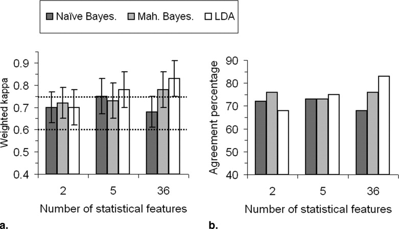
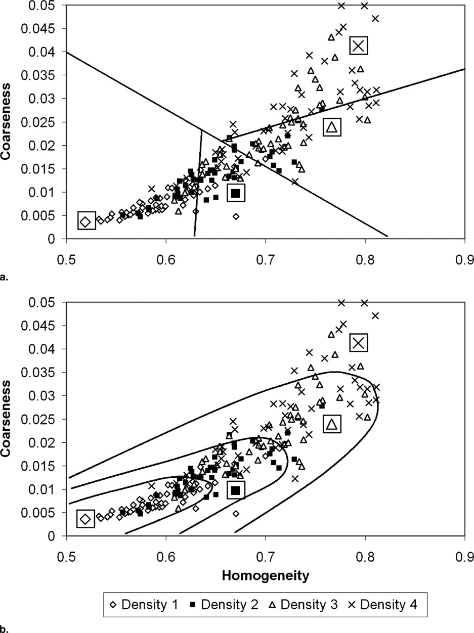
The proposed semiautomatic method makes use of complementary pattern recognition techniques to describe manually selected regions of interest (ROIs) in the breast with 36 statistical features. Three different classifiers based on a linear discriminant analysis or Bayesian theories were designed and tested on a database consisting of 1408 ROIs from 88 patients, using a leave-one-ROI-out technique. Classifications in optimal feature subspaces with lower dimensionality and reduction to a two-class problem were studied as well.

Results

Comparison with a reference established by the classifications of three radiologists shows excellent performance of the classifiers, even though extremely dense breasts continue to remain more difficult to classify accurately. For the two best classifiers, the exact agreement percentages are 76% and above, and weighted κ values are 0.78 and 0.83. Furthermore, classification in lower dimensional spaces and two-class problems give excellent results.

Conclusion

The proposed semiautomatic classifiers method provides an objective and reproducible method for characterizing breast density, especially for the two-class case. It represents a simple and valuable tool that could be used in screening programs, training, education, or for optimizing image processing in diagnostic tasks.

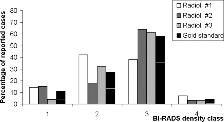
While the etiology of breast cancer remains unclear, many studies have demonstrated a correlation between cancer risk and factors such as age, breastfeeding and pregnancy history, family history of breast cancer, hormonal treatments, genetic factors, and breast density ( ). Breast density as a factor of risk was first investigated by Wolfe ( ), who defined a four-grade density scale on the basis of the patterns and textures observed on mammograms. Later, the BI-RADS (Breast Imaging Reporting Data System) density scale was developed by the American College of Radiology to standardize mammography reporting terminology and assessment and recommendation categories ( ). The BI-RADS density classification was created to inform referring physicians about the decline in sensitivity of mammography with increasing breast density. BI-RADS defines breast density 1 as almost entirely fatty, density 2 as scattered fibroglandular tissue, density 3 as heterogeneously dense tissue and density 4 as extremely dense tissues. It was not intended to serve as a method of measuring breast density percentage, although as per Wolfe’s scale ( ), correlations with this more objective factor do exist ( ). In clinical American and European conditions, the breast density of a given patient is typically evaluated and reported by a radiologist using BI-RADS on the basis of the simultaneous display of two mammograms per breast.

However, one of the difficulties for correctly assessing breast density is that the BI-RADS density scale definitions are rather subjective. A certain interpretational freedom prevents perfect interobserver and even intraobserver reproducibility ( ). On the other hand, numerous pattern recognition and classification techniques have been developed and can be directly applied to this task ( ). This is why different statistical approaches have been explored in the last few years in order to develop an objective classifier of mammograms according to Wolfe or the BI-RADS scale. These techniques have made use of various pattern recognition parameters to statistically describe the whole breast or part of it: fractal dimension ( ), gray level histogram properties ( ), moments ( ), gray level variations matrices ( ), or maximum response filters ( ). These descriptions have been combined with several general classification algorithms: Bayesian classification ( ), linear discriminant analysis (LDA) ( ), nearest neighbor rules ( ), neural networks, and textons ( ).

Get Radiology Tree app to read full this article<

Materials and methods

Mammogram Database

Get Radiology Tree app to read full this article<

Selection of Regions of Interest

Get Radiology Tree app to read full this article<

Statistical Description

Get Radiology Tree app to read full this article<

Table 1

Summary of the Texture Analysis Methods and the Corresponding Features

Analysis Method Statistical Features Gray level histogram standard deviation skewness kurtosis balance Gray level co-occurrence matrices energy entropy cmax contrast homogeneity Primitives matrices short primitive emphasis long primitive emphasis gray level uniformity primitive length uniformity Fractal analysis fractal dimension Neighbourhood gray-tone difference matrix

The 18 parameters in this table were computed for two scales as described in the text, making a total of 36 features.

Get Radiology Tree app to read full this article<

Definition of Gold Standard From Radiologists’ Ratings

Get Radiology Tree app to read full this article<

Classification Algorithms

Get Radiology Tree app to read full this article<

Classic Bayesian classifier based on Mahalanobis distance

Get Radiology Tree app to read full this article<

ψk(v)=1(2π)NdetKk√⋅exp[−12(v−μk)TK−1k(v−μk)], ψ

(

)

(

)

det

⁡

⋅

exp

⁡

[

−

(

−

)

−

(

−

)

]

where μ k represents the mean vector of class k and K k is the covariance matrix of vectors in class k :

μk=1nk∑vi∈Skvi μ

∑

∈

Kk=1nk−1∑vi∈Sk(vi−μk)T(vi−μk) K

−

∑

∈

(

−

)

(

−

)

Get Radiology Tree app to read full this article<

p(k∣∣v)=p(v|k)p(k)p(v)=ψk(v)pa(k)∑kψk(v)pa(k) p

(

)

(

)

(

)

(

)

(

)

(

)

∑

(

)

(

)

Get Radiology Tree app to read full this article<

cR=∑4k=1k⋅p(k|v), c

∑

⋅

(

)

with c R being rounded to the nearest integer value to obtain the class attributed to the tested sample vector v.

Get Radiology Tree app to read full this article<

pa(k)=14, p

(

)

which represents the most conservative a priori assumption.

Get Radiology Tree app to read full this article<

Naïve Bayesian classifier

Get Radiology Tree app to read full this article<

ψk(vn,k)=1(2π)N√exp[−12vTn,kvn,k], ψ

(

)

(

)

exp

⁡

[

−

]

where v has been normalized in the same way as training samples of class k to obtain the normalized vector v n,k . The four a posteriori probabilities p( k |v) were then computed with Equation 4 , and the attributed class with Equation 5 .

Get Radiology Tree app to read full this article<

12π√∫−∞pj,kne−t2/2dt=pj,kpj,kmax, 1

∫

−

∞

−

max

⁡

where p j,k max is the highest value in the original distribution of feature j in class k .

Get Radiology Tree app to read full this article<

Linear discriminant analysis

Get Radiology Tree app to read full this article<

ψk(v)=1(2π)NdetKo√⋅exp[−12(v−μk)TK−1o(v−μk)] ψ

(

)

(

)

det

⁡

⋅

exp

⁡

[

−

(

−

)

−

(

−

)

]

Get Radiology Tree app to read full this article<

Averaging the individual ROIs classifications

Get Radiology Tree app to read full this article<

Reduction of the features’ space size and number of classes

Get Radiology Tree app to read full this article<

Evaluation of the performance

Get Radiology Tree app to read full this article<

κ=po−pe1−pe, κ

−

where p o is the observed agreement proportion and p e the agreement expected by chance alone. Both are calculated from the confusion matrix and the quadratic weights matrix, and the values of κ stand between −1 and 1 (the minimum value actually depends on p e but is always between −1 and 0). Benchmarks by Landis and Koch ( ) (adjusted by Fleiss et al. [41] for taking the weighting process into account) are commonly used: κ values below 0.4 reflect poor agreement, between 0.4 and 0.6 moderate agreement, while it is substantial between 0.6 and 0.75 and excellent above 0.75. Weighted κ is particularly well adapted to multiclass tasks and when the classes are rather subjectively defined, which is the case for the BI-RADS density scale. The weighting process indeed differentiates between serious (more than one BI-RADS class difference) and slight disagreement (immediate neighbor class choice), and has been chosen as an evaluation parameter in numerous previous works on mammogram classification ( ). Although much more sensitive to differences in class prevalence, the exact agreement proportion was also computed to be able to compare the performance with results from other studies ( ).

Get Radiology Tree app to read full this article<

Results

Get Radiology Tree app to read full this article<

Table 2

Radiologist Classifications Compared to the Gold Standard Classification Defined in Text

Radiologist # 1 Radiologist # 2 Radiologist # 3 Kappa 0.81 ± 0.07 0.88 ± 0.07 0.91 ± 0.08 Exact agreement 77% 89% 89%

Standard error for weighted κ was computed according to the formula given by Fleiss et al. ( ).

Get Radiology Tree app to read full this article<

Table 3

(a) Confusion Matrix Obtained for the Bayesian Classifier Based on Mahalanobis Distance. Results are Averaged Over Mammogram Pairs from the Same View. (b) Same for LDA Classifier

(a) Gold Standard Bayesian Classifier Density 1 Density 2 Density 3 Density 4 Density 1 14 3 0 0 Density 2 5 30 6 1 Density 3 0 14 86 3 Density 4 0 0 10 4

(b) Gold Standard LDA Classifier Density 1 Density 2 Density 3 Density 4 Density 1 16 3 0 0 Density 2 3 31 4 1 Density 3 0 13 95 3 Density 4 0 0 3 4

Table 4

Weighted κ Values Obtained with the Different Averaging Processes and Classifiers. Exact Agreement is Given in Parenthesis

Individual ROI Classification Average per Mammogram (4 ROIs) Average per View Type (8 ROIs) Naïve Bayesian 0.50 ± 0.02 (39%) 0.65 ± 0.05 (55%) 0.68 ± 0.07 (60%) Mahalanobis Bayesian 0.58 ± 0.03 (53%) 0.73 ± 0.05 (69%) 0.78 ± 0.07 (76%) LDA 0.71 ± 0.03 (70%) 0.81 ± 0.05 (80%) 0.83 ± 0.08 (83%)

Get Radiology Tree app to read full this article<

Discussion

Get Radiology Tree app to read full this article<

Conclusion

Get Radiology Tree app to read full this article<

Acknowledgments

Get Radiology Tree app to read full this article<

Appendix

Definition of the statistical parameters

Parameters Computed From the Gray Level Histogram

Get Radiology Tree app to read full this article<

mean≡x¯=1N∑ixi mean

≡

∑

standarddev.≡σ=1N−1√(∑i(xi−x¯)2)1/2 standard

dev

≡

−

(

∑

(

−

)

skewness=1Nσ3∑i(xi−x¯)3 skewness

∑

(

−

)

kurtosis=1Nσ4∑i(xi−x¯)4−3 kurtosis

∑

(

−

)

−

balance=x70−x¯x¯−x30, balance

−

where the summations are performed over the N pixels of the ROI, and x p is the gray level yielding to p th percentile of the gray level distribution ( ).

Get Radiology Tree app to read full this article<

Gray Level Co-occurrence Matrices (GLCM)

Get Radiology Tree app to read full this article<

energy(C)=∑i,jC2i,j energy

(

)

∑

entropy(C)=−∑i,jCi,jlogCi,j entropy

(

)

−

∑

log

⁡

cmax(C)=maxi,jCi,j c

max

(

)

max

⁡

contrast(C)=∑i,j|i−j|2Ci,j contrast

(

)

∑

−

homogeneity(C)=∑i,jCi,j1+|i−j| homogeneity

(

)

∑

−

Get Radiology Tree app to read full this article<

Primitives Matrix (PM)

Get Radiology Tree app to read full this article<

spe=1Btot∑a∑rBa,rr2 spe

∑

lpe=1Btot∑a∑rBa,rr2 lpe

∑

glu=1Btot∑a(∑rBa,r)2 glu

∑

(

∑

)

plu=1Btot∑r(∑aBa,r)2, plu

∑

(

∑

)

where Btot is the sum of the elements of the primitives matrix B : Btot=∑a∑rBa,r. B

∑

. Note that B could be defined for several directions, but we limited our investigations to one ( ), corresponding to a scan of the image along direction [1,0].

Get Radiology Tree app to read full this article<

Fractal Dimension

Get Radiology Tree app to read full this article<

L(ε)=λε1−D L

(

)

−

Get Radiology Tree app to read full this article<

A(ε)=λε2−D A

(

)

−

Get Radiology Tree app to read full this article<

Neighborhood Gray-Tone Difference Matrix (NGTDM)

Get Radiology Tree app to read full this article<

A¯¯¯xk,l=1W−1[∑dm=−d∑dn=−dxk+m,l+n],(m,n)≠(0,0), A

−

[

∑

−

∑

−

]

(

)

≠

(

)

where d = 3 is the neighbouring size and W = (2d+1) 2 . Denoting { X i } the set of all pixels with value i in the ROI, the i th entry of the NGTDM is given by:

s(i)=∑x∈Xi∣∣i−A¯¯¯x∣∣ s

(

)

∑

∈

−

Get Radiology Tree app to read full this article<

coarseness=[ε+∑imaxi=0pis(i)]−1 c

[

∑

max

⁡

(

)

]

−

contrast′=[1Ng(Ng−1)∑imaxi=0∑jmaxj=0pipj(i−j)2]⋅[1n2∑imaxi=0s(i)] contrast

′

[

(

−

)

∑

max

⁡

∑

max

⁡

(

−

)

]

[

∑

max

⁡

(

)

]

complexity=∑imaxi=0∑jmaxj=0|i−j|[pis(i)+pjs(j)]n2(pi+pj),pi>0,pj>0 complexity

∑

max

⁡

∑

max

⁡

−

[

(

)

(

)

]

(

)

strength=∑imaxi=0∑jmaxj=0(pi+pj)(i−j)2ε+∑imaxi=0s(i),pi>0,pj>0, strength

∑

max

⁡

∑

max

⁡

(

)

(

−

)

∑

max

⁡

(

)

where pi=|Xi|/∑imaxi=0|Xi| p

∑

max

⁡

| is the probability of occurrence of gray level i in the ROI, i max the highest gray level and N g the number of different gray levels effectively present in the ROI and ε a small number (10 −12 in our case) to prevent coarseness and strength becoming infinite. The feature representing the contrast given by Equation 30 is called here contrast′ , to make a distinction with the contrast derived from the primitives matrices (see Equation 19 ).

Get Radiology Tree app to read full this article<

References

1. Fitzgibbons P.L., Page D.L., Weaver D., et. al.: Prognostic factors in breast cancer. Arch Pathol Lab Med 2000; 124: pp. 966-978.
2. Ziv E., Smith-Bindman R., Kerlikowske K.: Mammographic breast density and family history of breast cancer. J Natl Cancer Inst 2003; 95: pp. 556-558.
3. Colditz G.A., Hankison S.E., Hunter D.J., et. al.: The use of estrogens and progestins and the risk of breast cancer in postmenopausal women. N Engl J Med 1995; 332: pp. 1589-1593.
4. Kelsey J.L., Gammon M.D., John E.M.: Reproductive factors and breast cancer. Epidemiol Rev 1993; 15: pp. 36-47.
5. Boyd N.F., Byng J.W., Long R.A., et. al.: Quantitative classification of mammographic densities and breast cancer risk: Results from the Canadian National Breast Screening study. J Natl Cancer Inst 1995; 87: pp. 670-675.
6. van Gils C.H., Hendriks J.H., Holland R., et. al.: Changes in mammographic breast density and concomitant changes in breast cancer risk. Eur J Cancer Prev 1999; 8: pp. 509-515.
7. Heine J.J., Malhotra P.: Mammographic tissue, breast cancer risk, serial image analysis, and digital mammography: Part 1. Acad Radiol 2001; 9: pp. 298-316.
8. Wolfe J.N.: Breast patterns as an index of risk for developing breast cancer. AJR Am J Roentgenol 1976; 126: pp. 1130-1137.
9. American College of Radiology (ACR) 2004: ACR Practice Guideline for the performance of screening mammography.2004.
10. Harvey J.A., Bovbjerg V.E.: Quantitative assessment of mammographic breast density: relationship with breast cancer risk. Radiology 2004; 230: pp. 29-41.
11. Brisson J., Diorio C., Mâsse B.: Wolfe’s parenchymal pattern and percentage of the breast with mammographic densities: Redundant or complementary classifications?. Cancer Epidemiol Biomark Prevent 2003; 12: pp. 728-732.
12. Perconti P., Loew M.: Analysis of parenchymal patterns using conspicuous spatial frequency features in mammograms applied to the BI-RADS density rating scheme.2006.
13. Kerlikowske K., Grady D., Barclay J., et. al.: Variability and accuracy in mammographic interpretation using the American College of Radiology Breast Imaging Reporting and Data System. J Natl Cancer Inst 1998; 90: pp. 1801-1809.
14. Berg W.A., Campassi C., Langenberg P., Sexton M.J.: Breast Imaging Reporting and Data System: Inter- and intraobserver variability in feature analysis and final assessment. AJR Am J Roentgenol 2000; 174: pp. 1769-1777.
15. Huo Z., Giger M.L., Wolverton D.E., Zhong W., Cumming S., Olopade O.I.: Computerized analysis of mammographic parenchymal patterns for breast cancer assessment: Feature selection. Med Phys 2000; 27: pp. 4-12.
16. Caldwell C.B., Stappelton S.J., Holdsworth D.W., et. al.: Characterisation of mammographic parenchymal pattern by fractal dimension. Phys Med Biol 1990; 35: pp. 235-247.
17. Byng J.W., Boyd N.F., Fishel E., Jong R.A., Yaffe M.J.: Automated analysis of mammographic densities. Phys Med Biol 1996; 41: pp. 909-923.
18. Bovis K., Singh S.: Classification of mammographic breast density using a combined classifier paradigm. Proceedings of the 4th International Workshop on Digital Mammography 2002; pp. 177-180.
19. Zhou C., Chan H.P., Petrick N., et. al.: Computerized image analysis: Estimation of breast density on mammograms. Med Phys 2001; 28: pp. 1056-1569.
20. Tahoces P.G., Correa J., Souto M., Gómez L., Vidal J.J.: Computer-aided diagnosis: The classification of mammographic breast parenchymal patterns. Phys Med Biol 1995; 40: pp. 103-117.
21. Karssemeijer N.: Automated classification of parenchymal patterns in mammograms. Phys Med Biol 1998; 43: pp. 365-378.
22. Petroudi S., Kadir T., Brady M.: Automatic classification of mammographic parenchymal patterns: A statistical approach. Proc IEEE Int Conf Eng Med Biol 2003; pp. 798-801.
23. Vedantham S., Karellas A., Suryanarayanan S., et. al.: Full breast digital mammography with an amorphous silicon-based flat panel detector: Physical characteristics of a clinical prototype. Med Phys 2000; 27: pp. 558-567.
24. Burgess A.: On the noise variance of a digital mammography system. Med Phys 2004; 31: pp. 1987-1995.
25. Muller S.: Full-field digital mammography designed as a complete system. Eur J Radiol 1999; 31: pp. 25-34.
26. Hemdal B., Andersson I., Grahn A., et. al.: Can the average glandular dose in routine digital mammography screening be reduced?. Radiat Protect Dosimetry 2005; 114: pp. 383-388.
27. Li H., Giger M.L., Olopade O.I., Margolis A., Lan L., Chinander M.R.: Computerized texture analysis of mammographic parenchymal patterns of digitized mammograms. Acad Radiol 2005; 12: pp. 863-873.
28. Sonka M., Hlavak V., Boyle R.: Image processing.2nd ed.1999.Brooks/ColePacific Grove, CA
29. Tuceryan M., Jain A.K.: Texture analysis.Chen C.H.Pau L.F.Wang P.The Handbook of Pattern Recognition and Computer Vision.1998.World Scientific PublishingRiver Edge, NJ:
30. Haralick R.M., Shanmugam K., Dinstein I.: Textural features for image classification. IEEE Trans Syst Manage Cybern 1973; 3: pp. 610-662.
31. Lundhal T., Ohley W.J., Kunklinski W.S., Williams D.O., Gewirtz H., Most A.S.: Analysis and interpolation of angiographic images by use of fractals. Proceedings of IEEE Conference on Computers in Cardiology 1985; pp. 355-358.
32. Amadasun M., King R.: Textural features corresponding to textural properties. IEEE Trans Syst Manage Cybern 1989; 19: pp. 1264-1274.
33. Fukunaga K.: Introduction to Statistical Pattern Recognition.2nd ed.1990.Academic PressSan Diego, CA
34. Chabat F., Guang-Zhong Y., Mansell D.M.: Obstructive lung diseases: Texture classification for differentiation at CT. Radiology 2003; 228: pp. 871-877.
35. Friedman N., Geiger D., Goldszmidt M.: Bayesian network classifier. Machine Learning 1997; 29: pp. 131-163.
36. Domingos P., Pazzani M.J.: On the optimality of the simple Bayesian classifier under zero-one loss. Machine Learning 1997; 29: pp. 103-130.
37. 2004.MathWorksNatick, MA
38. Nasri M., El Hitmy M.: Algorithme génétique et Critère de la Trace pour l’Optimisation du vecteur Attribut: Application à la Classification Supervisée des Images de Textures.2002.
39. Yeom S., Javidi B.: Three-dimensional distortion-tolerant object recognition using integral imaging. Optics Express 2004; 12: pp. 5795-5809.
40. Barrett H.H., Myers K.J.: Foundations of Image Science.2004.WileyHoboken, NJ
41. Fleiss J.L., Levin B., Paik M.C.: Statistical Rates and Proportions.3rd ed.2003.WileyHoboken, NJ
42. Ker M.: Issues in the use of kappa. Invest Radiol 1991; 26: pp. 78-83.
43. Kundel H.L.: Measurement of Observer Agreement. Radiology 2003; 228: pp. 303-308.
44. Kraemer H.C.: Extension of the kappa coefficient. Biometrics 1980; 36: pp. 207-216.
45. Kraemer H.C., Periyakoil V.S., Noda A.: Kappa coefficients in medical research.D’Agostino R.B.2004.WileyHoboken, NJ:
46. Landis J.R., Koch G.G.: The measurement of observer agreement for categorical data. Biometrics 1973; 33: pp. 671-679.
47. Petroudi S., Brady M.: Proceedings of the 8th International Workshop on Digital Mammography.Proceedings of the 8th International Workshop on Digital Mammography.2006.SpringerBerlin/Heidelberg:pp. 609-615.
48. Mandelbrot B.B.: The Fractal Geometry of Nature.1982.WH FreemanSan Francisco, CA

Semiautomatic Mammographic Parenchymal Patterns Classification Using Multiple Statistical Features

Rationale and Objectives

Materials and Methods

Results

Conclusion

Materials and methods

Mammogram Database

Selection of Regions of Interest

Statistical Description

Definition of Gold Standard From Radiologists’ Ratings

Classification Algorithms

Classic Bayesian classifier based on Mahalanobis distance

Naïve Bayesian classifier

Linear discriminant analysis

Averaging the individual ROIs classifications

Reduction of the features’ space size and number of classes

Evaluation of the performance

Results

Discussion

Conclusion

Acknowledgments

Appendix

Definition of the statistical parameters

Parameters Computed From the Gray Level Histogram

Gray Level Co-occurrence Matrices (GLCM)

Primitives Matrix (PM)

Fractal Dimension

Neighborhood Gray-Tone Difference Matrix (NGTDM)

References

Further Reading

Abstracts of Funded National Institutes of Health Grants (December)

Computer-Aided Diagnosis Scheme for Detection of Lacunar Infarcts on MR Images

Congresses, Conferences, Meetings, and Seminars