Semiautomatic Segmentation of Vertebrae in Lateral X-rays Using a Conditional Shape Model

Rationale and Objectives

Manual annotation of the full contour of the vertebrae in lateral x-rays for subsequent morphometry is time-consuming. The standard six-point morphometry is commonly used instead. It has been shown that the information from the complete contour improves the quality of the study. In this article, the six landmarks are given and the vertebrae are segmented taking advantage of that information. The result is a semiautomatic system in which the full contour is found with high precision, and that only requires a radiologist to mark six points per vertebra.

Materials and Methods

A shape model was built for both the six landmarks and the full contours of the vertebrae L1, L2, L3, and L4 of 142 patients. The distribution of the principal components of the full contour was then modeled as a Gaussian conditional distribution depending on the principal components of the six landmarks. The conditional mean was used as initialization for active shape model optimization, and the conditional variance was used to constrain the solution to plausible shapes.

Results

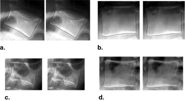
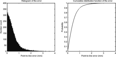
The achieved point-to-line error was 0.48 mm, and 95% of the points were located within 1.36 mm of the annotated contour. The accuracy is superior to those of previously published studies, at the expense of requiring the six points to be marked. Fractures and osteophytes are well approximated by the model, although they are sometimes oversmoothed.

Conclusions

The proposed method provides hence a richer description than the six points, and can be used as input for shape-based morphometry to detect and quantify vertebral deformation more accurately.

Osteoporosis is a disease of bone in which the bone mineral density is reduced, bone microarchitecture is disrupted, and the amount and variety of noncollagenous proteins in bone is altered ( ). Bones affected by the disease are more likely to fracture. Osteoporosis is defined by the World Health Organization as either a bone mineral density 2.5 standard deviations below peak bone mass (20-year-old, sex-matched healthy person average) as measured by dual x-ray absorptiometry (DXA), or any fragility fracture. Because of its hormonal component, more women, particularly after menopause, suffer from this disease than men.

Osteoporotic fractures are those that occur under slight amount of stress that would not normally lead to fractures in nonosteoporotic people. Typical fractures occur in the vertebral column, hip, and wrist. Vertebral fractures are the most common ones. They occur in younger patients and they are a good indicator for the risk of future spine and hip fractures. These two are the most serious cases, leading to limited mobility and possibly disability. Hip fracture, in particular, usually requires major surgery, which has important associated risks, such as deep vein thrombosis and pulmonary embolism. Although osteoporosis patients have an increased mortality rate because of the complications of fractures, most patients die with the disease rather than of it.

Get Radiology Tree app to read full this article<

Materials and methods

Available Data

Get Radiology Tree app to read full this article<

Methods

Get Radiology Tree app to read full this article<

1 Get Radiology Tree app to read full this article<

Get Radiology Tree app to read full this article<

2 Get Radiology Tree app to read full this article<

Get Radiology Tree app to read full this article<

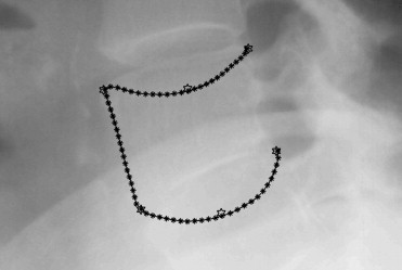
Landmark Placement

Get Radiology Tree app to read full this article<

Alignment

Get Radiology Tree app to read full this article<

x=[x1,x2,…,xN,y1,y2,…,yN]t x

[

…

]

Get Radiology Tree app to read full this article<

PDM

Get Radiology Tree app to read full this article<

x≈x¯+Pb x

≈

where b can be calculated for a certain shape:

b=Pt(x−x¯) b

(

−

)

and the approximation error vector is:

e=x−x¯−Pb=x−x¯−P(Pt(x−x¯)) e

−

(

−

)

where b is a column vector of k components, representing the projection of the shape onto the space of the model. Across the training set, the mean of this vector will be zero, and the covariance C will be a diagonal matrix including the k eigenvalues λ i .

Get Radiology Tree app to read full this article<

d=btC−b1−−−−−−√=∑ki=1(b2iλi)−−−−−−−−−√ d

−

∑

(

)

If the condition d < d max is not true, the b vector can be modified:

b′=b(dmax/d) b

′

⁢

(

)

Because the number of fractures in the dataset is low compared with the number of healthy ones, their influence on the model was increased by giving them a higher weight when building it. Two different weights were given to normal and fractured vertebrae when calculating the mean and the variance of the shapes, so that their total contributions were equal. Because 504 healthy and 64 fractured vertebrae were available, the weights were

Wh=12Nheal=0.5504 W

0.5

504

Wf=12Nfrac=0.564 W

0.5

x¯′=∑Nheali=1whxi+∑Nfracj=1wfxj x

′

∑

C′=Nheal+NfracNheal+Nfrac−1{∑Nheali=1wh(xi−x¯′)(xi−x¯′)t+∑Nfracj=1wf(xj−x¯′)(xj−x¯′)t} C

′

−

{

∑

(

−

′

)

(

−

′

)

∑

(

−

′

)

(

−

′

)

}

Get Radiology Tree app to read full this article<

Conditional Model

Get Radiology Tree app to read full this article<

P(F|L)=N(bcond,Ccond)bcond=μF+∑FL∑−1LL(L−μL)Ccond=∑FF−∑FL∑−1LL∑LF P

(

)

(

)

∑

−

(

−

)

∑

−

∑

−

∑

Get Radiology Tree app to read full this article<

ASM

Get Radiology Tree app to read full this article<

fi(t)=(pi(t)−p¯i)tS−1p,i(pi(t)−p¯i) f

(

)

(

)

−

)

−

(

)

−

)

where p ̶ i is the average of the profiles of length 2 T t + 1 around the points in the training cases, and S p,i is a diagonal matrix including the (independent) variances of each element in the profile. The function f i (t) will just be defined in the interval [− T p , T p ]. Therefore T p defines how far from the current point location the search for the contour is performed. If t m minimizes f i (t) , the shift 0.66 t m is chosen to make the algorithm evolve in a smoother way.

Get Radiology Tree app to read full this article<

(PtWs)dx=(PtWsP)db (

)

(

)

where W S is a diagonal matrix with weights that measure the importance of each point in the fitting. The weights depend on the magnitude of the displacement ( ) and on the goodness of the fit:

w′i=12+|dXi|21fi(tm) w

′

(

)

wi=w′i∑67l=1w′i w

′

∑

′

The idea behind the first term of the weight (2+|dXi|2)−1 (

)

−

1 is to prevent the shape model from fitting distant points that might be wrong, as least-squares is not robust against outliers. The second term ( f i ( t m )) −1 gives higher priority to fitting those points that are probably located on the right contour.

Get Radiology Tree app to read full this article<

btC−1b=∑ki=1(b2iλi) b

−

∑

(

)

does not hold any longer (even though it would be possible to diagonalize C cond and then use this simplification).

b′i+1=bi+db b

′

i+1

d=(b′i+1−bcond)tC−1cond(b′i+1−bcond)−−−−−−−−−−−−−−−−−−−−−−−−−−−√ d

(

′

−

)

−

(

′

−

)

and then

bi+1={b′i+1,bcond+(b′i+1−bcond)(dmax/d),ifd≤dmaxifd>dmax b

{

′

≤

max

⁡

(

′

−

)

(

max

⁡

)

max

⁡

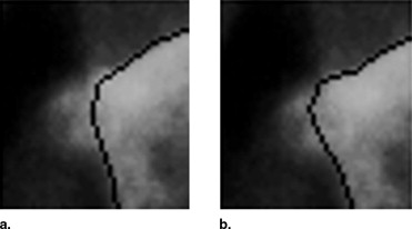
Therefore d max is the parameter that controls how free the algorithm is to fit the contour to the edges in the image. A large value allows the result to move around the principal component space, which can lead to implausible solutions if the edges are not clear in the image. A small value makes the algorithm rely mostly on the model, leading to more conservative solutions, closer to the mean of the distribution. This can prevent the algorithm from finding the correct solution, especially in abnormal cases with fractures or osteophytes, in which the real contour is relatively far from the initialization in the principal component space ( Fig 3 ).

Get Radiology Tree app to read full this article<

Results

Parameter Setting

Get Radiology Tree app to read full this article<

$Figure 5, Some samples from the leave-one-out experiments. For each pair, the image on the left represents the ground truth, while the one on the right represents the output of the algorithm. (a) Oversmoothing in fractured vertebra (0.85 mm mean point-to-line error), (b) wrong edge captured (0.83 mm), (c) well-segmented fracture (0.51 mm), and (d) typical, normal, well-segmented vertebra (0.33 mm).$

Get Radiology Tree app to read full this article<

Evaluation

Get Radiology Tree app to read full this article<

Discussion

Get Radiology Tree app to read full this article<

Table 1

Comparison of the Results from This Study and From the Literature

Authors Modality Error Measure Results Zamora et al X-rays Point-to-point average ≤6.4 mm (50% of cases) Smyth et al DXA Point-to-line RMS ≤1.23 in 95% of healthy ≤2.24 mm in 92% of fractures de Bruijne et al X-rays Point-to-line average 1.4 mm (healthy and fractures) Roberts et al DXA Point-to-line average 0.70 mm in healthy, 1.23 mm in fractures Roberts et al X-rays Point-to-line average 0.64 mm in healthy, 1.06 mm in fractures Roberts et al DXA Point-to-line average 0.69 mm in healthy, 0.96 mm in fractures This study X-rays Point-to-line average 0.47 mm in healthy, 0.54 mm in fractures

Get Radiology Tree app to read full this article<

Conclusion

Get Radiology Tree app to read full this article<

Acknowledgments

Get Radiology Tree app to read full this article<

References

1. Genant H.K., Guglielmi G., Jergas M.: Bone densitometry and osteoporosis.1997.SpringerBerlin
2. Black D.M., Palermo L., Nevitt M.C., et. al.: Comparison of methods for defining prevalent vertebral deformities: the Study of Osteoporotic Fractures. J Bone Miner Res 1995; 10: pp. 890-902.
3. Genant H.K., Wu C.Y., van Kuijk C., et. al.: Vertebral fracture assessment using a semiquantitative technique. J Bone Miner Res 1993; 8: pp. 1137-1148.
4. McCloskey E.V., Spector T.D., Eyres K.S., et. al.: The assessment of vertebral deformity: a method for use in population studies and clinical trials. Osteoporos Int 1993; 3: pp. 138-147.
5. Ferrar L., Jiang G., Admas J., et. al.: Identification of vertebral fractures: an update. Osteoporos Int 2005; 16: pp. 717-728.
6. Smyth P., Taylor C., Adams J.: Vertebral shape: automatic measurement with active shape models. Radiology 1999; 211: pp. 571-578.
7. Zamora G., Sari-Sarrafa H., Long R.: Hierarchical segmentation of vertebrae from X-ray images.Sonka M.Fitzpatrick M.Medical Imaging: Image Process.2003.Proc SPIE, SPIE Presspp. 631-642. 5302
8. de Bruijne M., Nielsen M.: Image segmentation by shape particle filtering.Kittler J.Petrou M.Nixon M.ICPR, IEEE Computer Society Press.2004.pp. 722-725. (III)
9. de Bruijne M., Lund M.T., Pettersen P.C., et. al.: Quantitative vertebral morphometry using neighbor-conditional shape models.Larsen R.Nielsen M.Sporring J.2006.pp. 1-8. MICCAI. Volume 4190 of LNCS, Springer
10. Roberts M.G., Cootes T.F., Adams J.E.: Vertebral shape: automatic measurement with dynamically sequenced active appearance models.Duncan J.Gerig G.2005.pp. 733-740. MICAAI. Volume 3750 of LNCS, Springer
11. Roberts M.G., Cootes T.F., Adams J.E.: Automatic segmentation of lumbar vertebrae on digitised radiographs using linked active appearance models. Proc Med Image Understanding Analysis 2006; 1: pp. 120-124.
12. Roberts M.G., Cootes T.F., Adams J.E.: Improving the segmentation accuracy of fractured vertebrae with dynamically sequenced active appearance models.2006.pp. 1-8.
13. Goodall C.R.: Procrustes methods in the statistical analysis of shape. J R Stat Soc 1991; 53: pp. 285-339.
14. Cootes T., Taylor C., Cooper D., et. al.: Active shape models—their training and application. Comput Vis Image Underst 1995; 61: pp. 38-59.
15. Cootes T., Taylor C., Lanitis D.H., et. al.: Building and using flexible models incorporating grey-level information. Proce Fourth Int Conf Computer Vision 1993; pp. 242-246.
16. Long L.R., Antani S., Lee D.J., et. al.: Biomedical information from a national collection of spine x-rays: film to content-based retrieval. Proceedings of the SPIE 2003; 5033: pp. 70-84.
17. Davies R.H., Twining C.J., Cooter T.F., et. al.: A minimum description length approach to statistical shape modeling. IEEE Trans Med Imaging 2002; 21: pp. 525-537.
18. Thodberg H.H.: Minimum description length shape and appearance models. Proc Inf Process Med Imaging 2003; 18: pp. 51-62.

Semiautomatic Segmentation of Vertebrae in Lateral X-rays Using a Conditional Shape Model

Rationale and Objectives

Materials and Methods

Results

Conclusions

Materials and methods

Available Data

Methods

Landmark Placement

Alignment

PDM

Conditional Model

ASM

Results

Parameter Setting

Evaluation

Discussion

Conclusion

Acknowledgments

References

Further Reading

3D Shape Analysis of the Supraspinatus Muscle

A Computer-Based Radiology Simulator as a Learning Tool to Help Prepare First-Year Residents for Being On Call

A Review of Research Into the Development of Radiologic Expertise Implications for Computer-Based Training