
Rationale and Objectives
Semiparametric methods provide smooth and continuous receiver operating characteristic (ROC) curve fits to ordinal test results and require only that the data follow some unknown monotonic transformation of the model’s assumed distributions. The quantitative relationship between cutoff settings or individual test-result values on the data scale and points on the estimated ROC curve is lost in this procedure, however. To recover that relationship in a principled way, we propose a new algorithm for “proper” ROC curves and illustrate it by use of the proper binormal model.
Materials and Methods
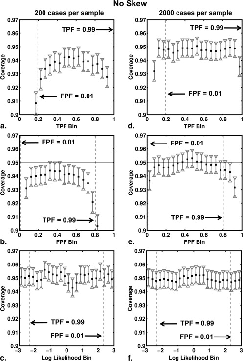
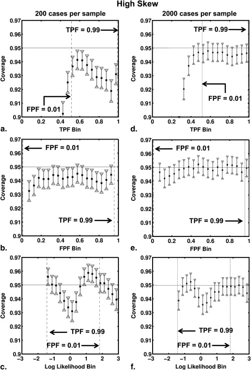
Several authors have proposed the use of multinomial distributions to fit semiparametric ROC curves by maximum-likelihood estimation. The resulting approach requires nuisance parameters that specify interval probabilities associated with the data, which are used subsequently as a basis for estimating values of the curve parameters of primary interest. In the method described here, we employ those “nuisance” parameters to recover the relationship between any ordinal test-result scale and true-positive fraction, false-positive fraction, and likelihood ratio. Computer simulations based on the proper binormal model were used to evaluate our approach in estimating those relationships and to assess the coverage of its confidence intervals for realistically sized datasets.
Results
In our simulations, the method reliably estimated simple relationships between test-result values and the several ROC quantities.
Conclusion
The proposed approach provides an effective and reliable semiparametric method with which to estimate the relationship between cutoff settings or individual test-result values and corresponding points on the ROC curve.
A receiver operating characteristic (ROC) curve is a continuous curve that plots sensitivity, often called true-positive fraction (TPF), as a function of 1 – specificity, here called false-positive fraction (FPF), and has become one of the primary tools used to assess the performance of diagnostic tests that classify individuals into two groups . During initial phases of a clinical evaluation of such tests, the focus is often on the ROC curve itself rather than upon the relationship between test-result values and points on that ROC curve (ie, pairs of TPF and FPF). An ROC curve summarizes the ability of any device or decision process to classify disease in a binary way without reference to the relationship between test-result values to points on the curve. However, when one wants to employ the classifier in a clinical situation, it is necessary to understand how values of the test’s quantitative results relate to particular “operating points” on the ROC curve, because a quantitative diagnostic method usually cannot be applied without adopting a particular test-result value as a cutoff to separate domains of distinctly different action (eg, do nothing or order additional tests, as in screening mammography). A closely related but subtly distinct estimation task concerns the position on a given ROC curve at which the test-result value of an individual patient lies, which quantifies the extent to which classification of that particular patient is “easy” or “difficult” for the diagnostic test in question and can serve as a basis for calibrating radiologists’ and/or automated classifiers’ reporting scales. Therefore, this article describes a new approach to the task of estimating the quantitative relationship between individual patients’ test-result values and/or various cutoff settings on the test-result scale, on one hand, and position on the corresponding test’s ROC curve, on the other.
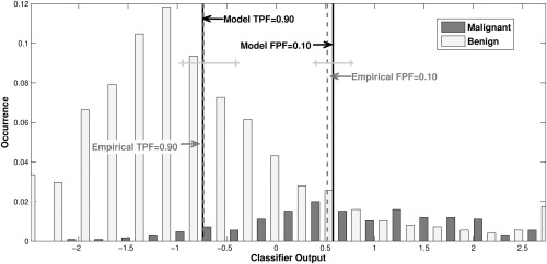
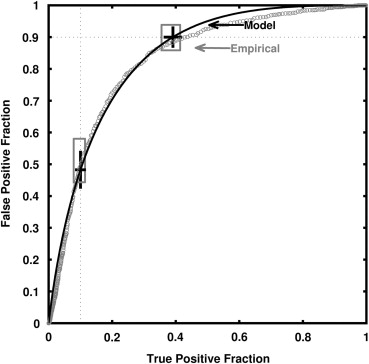
A concrete example may help to clarify one aspect of our motivation. Consider a computer classifier designed to diagnose breast cancer from mammographic images, the output of which lies on a scale from 0% to 100%, with larger values indicating stronger likelihood of the presence of malignancy. The ROC curve of such a classifier can be estimated from the test results of a sample of patients’ images by any of a variety of methods. However, most methods for ROC curve estimation cannot answer questions such as “What are the classifier’s sensitivity and specificity (ie, its ROC operating point) if every breast lesion with a computer output greater than 2% is sent to biopsy?” Here we address this need for “proper” (ie, convex) ROC curves, with primary focus on the proper binormal model.
Get Radiology Tree app to read full this article<
Get Radiology Tree app to read full this article<
Get Radiology Tree app to read full this article<
Get Radiology Tree app to read full this article<
Get Radiology Tree app to read full this article<
Materials and methods
Brief Description of the Ogilvie-Dorfman-Metz Approach to Estimation of ROC Curves
Get Radiology Tree app to read full this article<
Get Radiology Tree app to read full this article<
Get Radiology Tree app to read full this article<
n→0≡{n0,1,n0,2,…,n0,M|∑in0,i=N0} n
→
0
≡
{
n
0
,
1
,
n
0
,
2
,
…
,
n
0
,
M
|
∑
i
n
0
,
i
=
N
0
}
and for its N 1 actually positive cases (class 1):
n→1≡{n1,1,n1,2,…,n1,M|∑in1,i=N1}. n
→
1
≡
{
n
1
,
1
,
n
1
,
2
,
…
,
n
1
,
M
|
∑
i
n
1
,i
=
N
1
}
.
Get Radiology Tree app to read full this article<
Get Radiology Tree app to read full this article<
LLR∝∑i=1,Mn0,ilogp0,i+∑i=1,Mn1,ilogp1,i LLR
∝
∑
i
=
1
,
M
n
0
,
i
log
p
0
,
i
+
∑
i
=
1
,
M
n
1
,
i
log
p
1
,
i
where p 0, i and p 1, i are the probabilities associated with category i for the negative and positive distributions, respectively. These probabilities can be defined for a semiparametric model via the equations
p0,i=P(xi−1<x≤xi|α,β,−) p
0
,
i
=
P
(
x
i
−
1
<
x
≤
x
i
|
α
,
β
,
−
)
p1,i=P(xi−1<x≤xi|α,β,+), p
1
,i
=
P
(
x
i
−
1
<
x
≤
x
i
|
α
,
β
,
+
)
,
in which the parameters α and β specify a particular member of the population-model family (usually only two parameters are employed, to avoid overfitting) and x→ x
→ is a vector of ordinal category boundaries (“cutoffs”) on the latent decision-variable scale, x . Notice that each conditional-probability vector contains M-1 elements, because p 0,M and p 1,M are completely defined by its previous M-1 values, given that probabilities must sum to 1. Thus, the pairs (p0,i,p1,i) (
p
0
,
i
,
p
1
,
i
) are given by
P(xi−1<x≤xi|α,β,−)=∫xi−1xifx(x|α,β,−)dx P
(
x
i
−
1
<
x
≤
x
i
|
α
,
β
,
−
)
=
∫
x
i
−
1
x
i
f
x
(
x|
α
,
β
,
−
)
dx
and
P(xi−1<x≤xi|α,β,+)=∫xi−1xifx(x|α,β,+)dx, P
(
x
i
−
1
<
x
≤
x
i
|
α
,
β
,
+
)
=
∫
x
i
−
1
x
i
f
x
(
x|
α
,
β
,
+
)
dx
,
respectively, where fx(x|α,β,−) f
x
(
x
|
α
,
β
,
−
) and fx(x|α,β,+) f
x
(
x|
α
,
β
,
+
) are the model’s probability density functions for actually negative and actually positive cases, respectively. The task of maximum-likelihood estimation is to calculate the values of the parameters α, β and that maximize Equation 1 . From this point forward, we use the term MLE to indicate the Ogilvie-Dorfman-Metz semiparametric approach unless otherwise specified.
Get Radiology Tree app to read full this article<
Estimation of the Relationship between the Test-Result and the Latent Variable
Get Radiology Tree app to read full this article<
xˆ(ti)=x¯i≡n0,in0,i+n1,i∫xi-1xixfx(x|α,β,−)dx/∫xi−1xifx(x|α,β,−)dx+n1,in0,i+ni,1∫xi−1xixfx(x|α,β,+)dx/∫xi−1xifx(x|α,β,+)dx x
ˆ
(
t
i
)
=
x
¯
i
≡
n
0
,
i
n
0
,
i
+
n
1
,
i
∫
x
i-
1
x
i
x
f
x
(
x|
α
,
β
,
−
)
dx
/
∫
x
i
−
1
x
i
f
x
(
x|
α
,
β
,
−
)
dx
+
n
1
,
i
n
0
,i
+
n
i
,
1
∫
x
i
−
1
x
i
x
f
x
(
x|
α
,
β
,
+
)
dx
/
∫
x
i
−
1
x
i
f
x
(
x
|
α
,
β
,
+
)
dx
or the median
xˆ(ti)=x˜i≡μ1/2{n0,in0,i+n1,ifx(x|α,β,−)+n1,in0,i+n1,ifx(x|α,β,+)|xi−1<x<xi}, x
ˆ
(
t
i
)
=
x
˜
i
≡
μ
1
/
2
{
n
0
,
i
n
0
,
i
+
n
1
,
i
f
x
(
x|
α
,
β
,
−
)
+
n
1
,
i
n
0
,
i
+
n
1
,
i
f
x
(
x|
α
,
β
,
+
)
|
x
i
−
1
<
x
<
x
i
}
,
where μ1/2{f(x)|R} μ
1
/
2
{
f
(
x
)
|
R
} indicates the median of any probability density f(x) within the range R, and where x 0 and x M are defined as −∞ and +∞, respectively. The density in curly braces in Equation 4b is the estimate of the population mixture distribution that is associated with the conditional densities f x (x|α,β,−) and f x (x|α,β,+) within the interval x i < x < x i-1 .
Get Radiology Tree app to read full this article<
Get Radiology Tree app to read full this article<
LLR(ti)=LLRi=LLR(x˜i), LLR
(
t
i
)
=
LL
R
i
=
LLR
(
x
˜
i
)
,
where LLR(x˜i) (
x
˜
i
) is determined analytically by the model. However, the mean of LLR is not the LLR of the mean, so when means are used to define the complimentary relationship between test-result and LLR, the mean value of LLR must be computed directly from the mixture distribution of the latent variable between the estimated cutoffs:
LLR(ti)=LLRi≡n0,in0,i+n1,i∫xi-1xiLLR(x)fx(x|α,β,−)dx/∫xi−1xifx(x|α,β,−)dx+n1,in0,i+ni,1∫xi−1xiLLR(x)fx(x|α,β,+)dx/∫xi−1xifx(x|α,β,+)dx. LLR
(
t
i
)
=
LL
R
i
≡
n
0
,
i
n
0
,
i
+
n
1
,
i
∫
x
i-
1
x
i
LLR
(
x
)
f
x
(
x|
α
,
β
,
−
)
dx
/
∫
x
i
−
1
x
i
f
x
(
x|
α
,
β
,
−
)
dx
+
n
1
,
i
n
0
,
i
+
n
i
,
1
∫
x
i
−
1
x
i
LLR
(
x
)
f
x
(
x|
α
,
β
,
+
)
dx
/
∫
x
i
−
1
x
i
f
x
(
x|
α
,
β
,
+
)
dx
.
Get Radiology Tree app to read full this article<
Get Radiology Tree app to read full this article<
Get Radiology Tree app to read full this article<
TPF(ti)≡TPF(x˜i)FPF(ti)≡FPF(x˜i), TPF
(
t
i
)
≡
TPF
(
x
˜
i
)
FPF
(
t
i
)
≡
F
PF
(
x
˜
i
)
,
where, as was the case with LLR, TPF(t i ) and FPF(t i ) are determined analytically from the median value within a range on the latent scale of an assumed model. Note that the operating point ( FPF(t i ), TPF(t i ) ) lies on the estimated ROC curve, and that LLR(t i ) is the natural (Napierian) logarithm of the slope of the estimated curve at that point.
Get Radiology Tree app to read full this article<
Get Radiology Tree app to read full this article<
Get Radiology Tree app to read full this article<
Description of the Simulation Studies
Get Radiology Tree app to read full this article<
v=(b+1)ya+a2+2(1−b2)y√, v
=
(
b
+
1
)
y
a
+
a
2
+
2
(
1
−
b
2
)
y
,
where
y=LLR−log(b) y
=
LLR
−
log
(
b
)
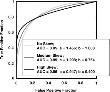
and where a and b are the conventional binormal parameters . (Notice that we are expressing the proper binormal model here in terms of the conventional binormal parameters a and b rather than the usual proper-binormal parameters d a and c , because doing so simplifies this discussion somewhat; however, readers must keep in mind that we are discussing the proper binormal model here.) From each of three population density pairs, the binormal parameters and ROC curves of which are shown in Figure 1 , we generated 5000 datasets of 200, 300, 400, and 1000 values of v . The skewed curves that we simulated cling only to the FPF = 0 axis rather than to the TPF = 1 axis because previous simulation studies showed that curves clinging to TPF = 1 behave identically due to model symmetries , as expected. The prevalence of actually positive cases was 50% for each simulated dataset. For each input test-result value, our algorithm estimated the corresponding TPF, FPF, and LLR values together with the uncertainties of these estimates.
Get Radiology Tree app to read full this article<
Get Radiology Tree app to read full this article<
y=2v(a+(1−b)v)1+b, y
=
2
v
(
a
+
(
1
−
b
)
v
)
1
+
b
,
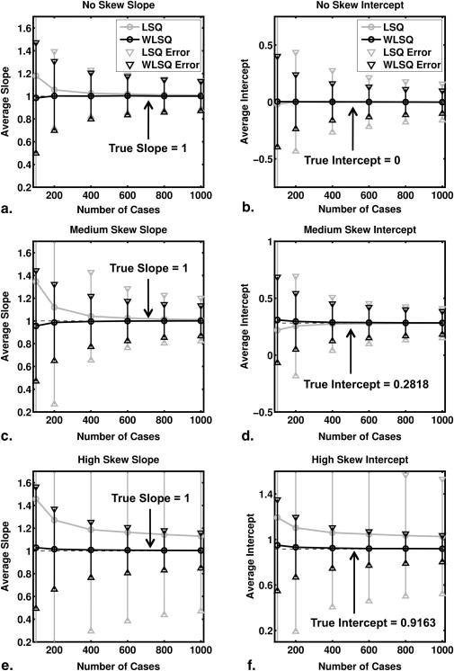
which is the inverse of Equation 8 . Thus, the transformed test-result values are linearly related to the true LLR by Equation 9 , so linear regression of the transformed test-result values y and estimated LLR produced estimates of the regression slope and intercept with true values 1 and -log(b), respectively. Note that in this case a linear relationship is the true model rather than an approximation. We used both ordinary and weighted least squares regression, with the reciprocal of the errors on the estimated LLR provided by the delta method as weights in the latter.
Get Radiology Tree app to read full this article<
Get Radiology Tree app to read full this article<
σ(Ck)=Ck(1−Ck)Nk−1−−−−−−−√, σ
(
C
k
)
=
C
k
(
1
−
C
k
)
N
k
−
1
,
where C k is the coverage for 95% CI of the kth bin and N k is the number of datasets with at least one true value in the kth bin. This choice of N k derives from two observations. If many corresponding true values fall into a particular bin for a given dataset of v values, then the corresponding estimated values of FPF, TPF , and LLR will be highly correlated, so care must be taken to ensure that the large number of such highly correlated values does not overly effect (and therefore bias) the error estimate provided by Equation 10 , which implicitly assumes independent events. On the other hand, if none of the corresponding true values fall into a particular bin for a given dataset of v values, then that dataset should not be counted in the error estimation.
Get Radiology Tree app to read full this article<
Get Radiology Tree app to read full this article<
Description of the Real-data Analysis
Get Radiology Tree app to read full this article<
Get Radiology Tree app to read full this article<
Results
Get Radiology Tree app to read full this article<
Get Radiology Tree app to read full this article<
Get Radiology Tree app to read full this article<
Get Radiology Tree app to read full this article<
Get Radiology Tree app to read full this article<
Get Radiology Tree app to read full this article<
Get Radiology Tree app to read full this article<
Get Radiology Tree app to read full this article<
Get Radiology Tree app to read full this article<
Discussion
Get Radiology Tree app to read full this article<
Get Radiology Tree app to read full this article<
Get Radiology Tree app to read full this article<
Get Radiology Tree app to read full this article<
Get Radiology Tree app to read full this article<
Get Radiology Tree app to read full this article<
Get Radiology Tree app to read full this article<
References
1. Wagner R.F., Metz C.E., Campbell G.: Assessment of medical imaging systems and computer aids: a tutorial review. Acad Radiol 2007; 14: pp. 723-748.
2. Pepe M.S.: The statistical evaluation of medical tests for classification and prediction.2004.Oxford University PressOxford; New York
3. Zhou X.-H., Obuchowski N.A., McClish D.K.: Statistical methods in diagnostic medicine.2002.Wiley-InterscienceNew York
4. Diabetes. World Health Organization. Available from http://www.who.int/topics/diabetes_mellitus/en/ (accessed July 14, 2010).
5. American College of Radiology: Breast imaging reporting and data system (BI-RADS).2003.American College of RadiologyReston, VA
6. Kvam P.H., Vidakovic B.: Nonparametric statistics with applications to science and engineering.2007.Wiley-InterscienceHoboken, NJ
7. Hanley J.A.: Receiver operating characteristic (ROC) methodology: the state of the art. Crit Rev Diagn Imaging 1989; 29: pp. 307-335.
8. Swets J.A.: Form of empirical ROCs in discrimination and diagnostic tasks: implications for theory and measurement of performance. Psychol Bull 1986; 99: pp. 181-198.
9. Swets J.A.: Indices of discrimination or diagnostic accuracy: their ROCs and implied models. Psychol Bull 1986; 99: pp. 100-117.
10. Hanley J.A.: The robustness of the “binormal” assumptions used in fitting ROC curves. Med Decis Making 1988; 8: pp. 197-203.
11. Pesce L.L., Metz C.E.: Reliable and computationally efficient maximum-likelihood estimation of “proper” binormal ROC curves. Acad Radiol 2007; 14: pp. 814-829.
12. Metz C.E., Herman B.A., Shen J.H.: Maximum likelihood estimation of receiver operating characteristic (ROC) curves from continuously-distributed data. Stat Med 1998; 17: pp. 1033-1053.
13. Dorfman D.D., Alf E.: Maximum-likelihood estimation of parameters of signal-detection theory and determination of confidence intervals—rating method data. J Math Psychol 1969; 6: pp. 487-496.
14. Metz C.E.: Basic principles of ROC analysis. Semin Nucl Med 1978; 8: pp. 283-298.
15. Agresti A.: Categorical data analysis.2nd ed.2002.Wiley-InterscienceNew York
16. Wagner R.F., Beiden S.V., Metz C.E.: Continuous versus categorical data for ROC analysis: some quantitative considerations. Acad Radiol 2001; 8: pp. 328-334.
17. Yousef W.A., Kundu S., Wagner R.F.: Nonparametric estimation of the threshold at an operating point on the ROC curve. Comput Stat Data Anal 2009; 53: pp. 4370-4383.
18. Drukker K., Pesce L., Giger M.: Repeatability in computer-aided diagnosis: application to breast cancer diagnosis on sonography. Med Phys 2010; 37: pp. 2659-2669.
19. Fleiss J.L., Levin B.A., Paik M.C.: Statistical methods for rates and proportions.3rd ed.2003.WileyHoboken, NJ
20. Ogilvie J., Creelman C.D.: Maximum likelihood estimation of receiver operating characteristic curve parameters. J Math Psychol 1968; 5: pp. 377-391.
21. Papoulis A.: Probability, random variables, and stochastic processes.2nd ed.1984.McGraw-HillNew York
22. Kendall M.G., Stuart A., Ord J.K., et. al.: Kendall’s advanced theory of statistics.6th ed.1994.Edward Arnold; Halsted PressLondon, New York
23. Metz C.E., Pan X.: “Proper” binormal ROC curves: theory and maximum-likelihood estimation. J Math Psychol 1999; 43: pp. 1-33.
24. Horsch K., Giger M.L., Venta L.A., et. al.: Automatic segmentation of breast lesions on ultrasound. Med Phys 2001; 28: pp. 1652-1659.
25. Horsch K., Giger M.L., Venta L.A., et. al.: Computerized diagnosis of breast lesions on ultrasound. Med Phys 2002; 29: pp. 157-164.
26. Drukker K., Giger M.L., Vyborny C.J., et. al.: Computerized detection and classification of cancer on breast ultrasound. Acad Radiol 2004; 11: pp. 526-535.
27. Drukker K., Giger M.L., Metz C.E.: Robustness of computerized lesion detection and classification scheme across different breast US platforms. Radiology 2005; 237: pp. 834-840.
28. Efron B., Tibshirani R.: An introduction to the bootstrap.1993.Chapman & HallNew York
29. Horsch K., Giger M.L., Metz C.E.: Prevalence scaling: applications to an intelligent workstation for the diagnosis of breast cancer. Acad Radiol 2008; 15: pp. 1446-1457.
30. Horsch K, Pesce LL, Giger ML, et al. A scaling transformation for classifier output based on likelihood ratio: applications to a CAD workstation for diagnosis of breast cancer. Med Phys. In review.