Spatial Localization Accuracy of Radiologists in Free-Response Studies Inferring Perceptual FROC Curves from Mark-Rating Data

Rationale and Objectives

Free-response data consist of a set of mark-ratings pairs. Before analysis, the data are classified or “scored” into lesion and non-lesion localizations. The scoring is done by choosing an acceptance-radius and classifying marks within the acceptance-radius of lesion centers as lesion localizations, and all other marks are classified as non-lesion localizations. The scored data are plotted as a free-response receiver operating characteristic (FROC) curve, essentially a plot of appropriately normalized numbers of lesion localizations vs. non-lesion localizations. Scored FROC curves are frequently used to compare imaging systems and computer-aided detection (CAD) algorithms. However, the choice of acceptance-radius is arbitrary. This makes it difficult to compare curves from different studies and to estimate true performance.

Materials and Methods

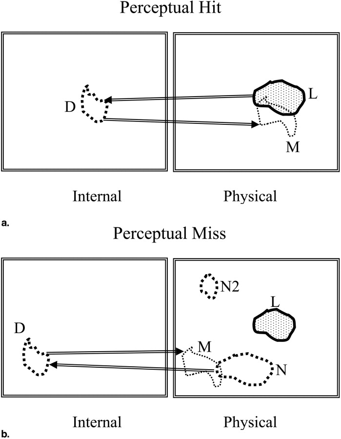
To resolve this issue the concept of two types of marks is introduced: perceptual hits and perceptual misses. A perceptual hit is a mark made in response to the observer seeing the lesion. A perceptual miss is a mark made in response to the observer seeing a (lesion-like) non-lesion. A method of estimating the most probable numbers of perceptual hits and misses is described. This allows one to plot a perceptual FROC operating point and by extension a perceptual FROC curve. Unlike a scored FROC operating point, a perceptual point is independent of the choice of acceptance-radius. The method does not allow one to identify individual marks as perceptual hits or misses—only the most probable numbers. It is based on a three-parameter statistical model of the spatial distributions of perceptual hits and misses relative to lesion centers.

Results

The method has been applied to an observer dataset in which mammographers and residents with different levels of experience were asked to locate lesions in mammograms. The perceptual operating points suggest superior performance for the mammographers and equivalent performance for residents in the first and second mammography rotations. These results and the model validation are preliminary as they are based on a small dataset.

Conclusion

The significance of this study is showing that it is possible to probabilistically determine if a mark resulted from seeing a lesion or a non-lesion. Using the method developed in this study one could perform acceptance-radius independent estimation of observer performance.

The free-response receiver operating characteristic (FROC) paradigm ( ) is being increasingly used in the assessment of medical imaging systems ( ), particularly in the evaluation of computer-aided detection (CAD) ( ) algorithms. The paradigm differs from the traditional receiver operating characteristic (ROC) method ( ) in that it seeks location information from the observer, rewarding the observer when the reported disease is marked in the appropriate location and penalizing the observer when it is not. This task is more relevant to the clinical practice of radiology, where it is not only important to identify disease, but also to offer further guidance regarding other characteristics (such as location) of the disease. In the FROC paradigm the data-unit is a mark-rating pair in which a variable number (0, 1, 2, …) of mark-rating pairs can occur on an image. A mark is the indicated location of a region that was considered worthy of reporting (ie, sufficiently suspicious) by the radiologist. The rating is a number representing the degree of suspicion, or confidence level, that the region in question is actually a lesion. In the ROC paradigm, the data-unit is a single rating per image and no location information is collected. Several methods of analyzing free-response data have been described ( ). All of these methods share a well-known weakness that is detailed in the following section.

Before FROC data can be analyzed, they need to be scored . Scoring refers to the investigator’s decision to classify each mark either as a lesion-localization (LL) or as a non-lesion localization (NL). (To avoid confusion with ROC studies, we avoid use of the terms true positives or false positives to describe the classification of marks.) The classification into LL or NL is done by adopting a closeness or proximity criterion. Intuitively, if a mark is close to a lesion, then it ought to be classified as an LL and, conversely, if it is far from any lesions it ought to be classified as an NL. However, what constitutes “close” is at the discretion of the investigator. In the past, researchers have used varying criteria to decide if a mark is close enough to be classified as an LL ( ). For example, any mark made within the boundary of a lesion could be considered an LL ( ). Another possibility is to select a distance criterion, termed acceptance-radius by us ( ), and if a mark falls within this distance of the center of a lesion, then it is classified as an LL and all other marks are classified as NLs. The choice of the acceptance-radius has an obvious effect on the observer’s performance. Choosing a larger acceptance-radius will increase the number of marks that are scored as LLs and decrease the number of NLs, thereby increasing apparent FROC observer performance. This work addresses the issue of how to resolve the arbitrariness of the choice of the acceptance-radius and its effect on performance measurement.

Get Radiology Tree app to read full this article<

Open full size image

Figure 1

The effect of choice of acceptance-radius (AR) on scored free-response receiver operating characteristic (FROC) curves. Shown are three scored FROC curves. The curve labeled “AR = medium” is for a moderate choice of AR. The curve labeled “AR = large” is for a larger choice of AR. It exhibits a higher plateau (more lesion localizations) and a smaller extent along the x-axis (fewer non-lesion localizations). The curve labeled “AR = small” has the opposite characteristics. These curves demonstrate the arbitrary nature of the scored FROC curve, and the consequent arbitrariness of the performance measurement.

Get Radiology Tree app to read full this article<

Materials and methods

Perceptual Hits and Misses

Get Radiology Tree app to read full this article<

Rationale for the Spatial Distribution Model for the Marks

Get Radiology Tree app to read full this article<

Mathematical Model for the Spatial Distribution of the Marks

Get Radiology Tree app to read full this article<

(r,σ)=12πσ2exp(−r22σ2).∫0∞2πr(r,σ)dr=1 (

)

exp

⁡

(

−

)

∫

∞

(

)

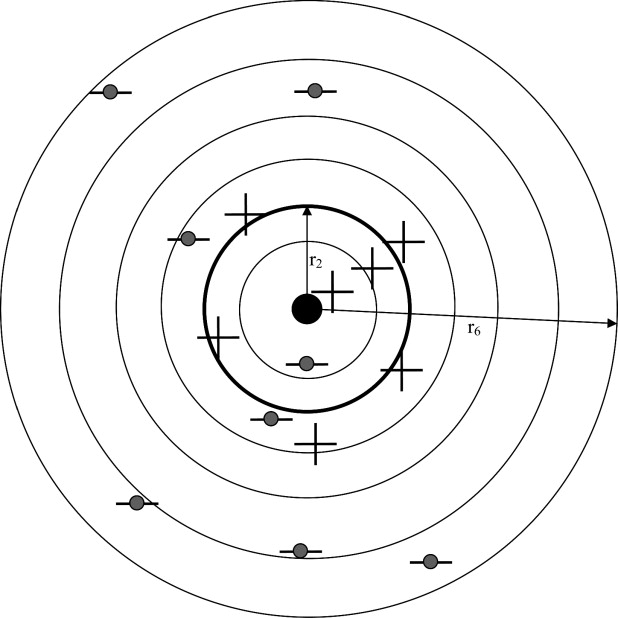
It is assumed that the spatial distribution of the marks can be modeled by a mixture distribution consisting of two Gaussians of the type described above with standard deviations σ 1 and σ 2 and mixing fraction α. The Gaussians with standard deviations σ 1 and σ 2 correspond to the perceptual hits and misses, respectively, and based on the preceding discussion one expects σ 1 « σ 2 (ie, the spread of the perceptual hits is smaller than that of the perceptual misses). Both Gaussians are centered at the common lesion center in the image stack, the solid dot in Fig 3 , which is defined as the origin of the coordinate system. If the distribution of the perceptual misses is broad, as will be seen to be true for our datasets, it does not matter where it is centered, and for simplicity in modeling we have assumed it is centered at the origin.

Get Radiology Tree app to read full this article<

r→=[r0,r1,…,rNB] r

→

[

…

]

where r 0 ≡ 0 and the bin denoted by r 1 is a circle of radius r 1 and the remaining bins are annuli with finite inner radii.

Get Radiology Tree app to read full this article<

fH(i∣∣∣α,σ1)=α∫ri−1ri2πr(r,σ1)drfM(i∣∣∣α,σ2)=(1−α)∫ri−1ri2πr(r,σ2)dr, f

(

)

∫

−

(

)

(

)

(

−

)

∫

−

(

)

where i = 1, 2, …, N B . It is assumed that rNB>>σ2>σ1 r



1 so that all of the integrated areas under the pdfs are included. For example:

α∫r0rNB2πr(r,σ1)dr=α(1−α)∫rorNB2πr(r,σ2)dr=1−α. α

∫

(

)

(

−

)

∫

(

)

−

Get Radiology Tree app to read full this article<

Determination of the Parameters

Get Radiology Tree app to read full this article<

N⃗ =[N1,N2,…,NNB], N

⃗

[

…

]

where Ni is the number of marks in bin i (eg, in Fig 3 , N 3 = 6). The probability of observing a mark in bin “i,” regardless of whether it is a hit or a miss, is given by

P(i|α,σ1,σ2)=fH(i|α,σ1)+fM(i|α,σ2). P

(

)

(

)

(

)

Assume that the numbers of marks Ni in the different bins are independent. The probability of observing the data vector N⃗ N

⃗ is given by (ignoring factors that are independent of the parameters σ 1 , σ 2 , and α)

P(N⃗ ∣∣α,σ1,σ2)=∏NBi=1[P(i|α,σ1,σ2)]Ni. P

(

⃗

)

∏

[

(

)

]

The total number of marks in the data set is N, where

N=∑NBi=1Ni. N

∑

The log-likelihood function is given by

LL≡LL(N→∣∣∣α,σ1,σ2)=∑NBi=1Nilog(P(i|α,σ1,σ2)). L

≡

(

→

)

∑

log

⁡

(

)

The parameters of this model, σ 1 , σ 2 , and α, can be determined by maximizing the log-likelihood function with respect to these parameters. In this work, we used the method of simulated annealing as implemented in the GNU library ( ) to minimize the negative of log-likelihood (−LL). The starting parameter values were σ 1 = 0.05, σ 2 = 2.0, and α = 0.8. The final estimates were insensitive to different choices of starting values, suggesting that the algorithm was not finding local minima. The covariance matrix is the inverse of the expectation value of the matrix of second partial derivatives of −LL with respect to the parameters, evaluated at the final parameter estimates ( ). The diagonal elements of the covariance matrix are the variances of the parameter estimates.

Get Radiology Tree app to read full this article<

Determination of the Most Probable Values of Perceptual Hits and Misses

Get Radiology Tree app to read full this article<

Ni=NHi+NMi N

Because of the stochastic nature of the problem, it is not possible to determine if any individual mark is a perceptual hit or a miss. The most probable number (an integer) of perceptual hits NHmax,i N

max

⁡

H in the i th bin can be determined as follows. The probability of observing NHi N

H perceptual hits in the i th bin is given by

P(NHi∣∣∣Ni,α,σ1,σ2)=Ni!NHi!(Ni−NHi)![fH(i|α,σ1)]NHi[fM(i|α,σ2)]Ni−NHi. P

(

)

(

−

)

[

(

)

]

[

(

)

]

−

This leads to the following expression for the log-likelihood function LL(NHi∣∣Ni,α,σ1,σ2) L

(

)

LL(NHi∣∣Ni,α,σ1,σ2)=−log[NHi!]−log[(Ni−NHi)!]+NHilog[fH(i|α,σ1)]+(Ni−NHi)log[fM(i|α,σ2)] L

(

)

−

log

⁡

[

]

−

log

⁡

[

(

−

)

]

log

⁡

[

(

)

]

(

−

)

log

⁡

[

(

)

]

where only terms involving NHi N

H , the quantity to be estimated, have been retained. The most probable value of NHi N

H can be found by determining the integer value of NHi N

H that yields the largest value of LL(NHi∣∣Ni,α,σ1,σ2) L

(

) , ie,

NHmax,i=argmaxNHi(LL(NHi∣∣Ni,α,σ1,σ2).) N

max

⁡

arg

⁡

max

⁡

(

)

Note that this maximization is performed using the values for σ 1 , σ 2 , and α determined previously. The corresponding value of NMmax,i N

max

⁡

M is Ni−NHmax,i N

−

max

⁡

H . The expected values of NHi N

H and NMi N

M are given by

⟨NHi⟩=N⋅fH(i∣∣α,σ1), 〈

〉

(

and

⟨NMi⟩=N⋅fM(i∣∣α,σ2). 〈

〉

(

These values will in general be non-integers and will satisfy

∑NBi=1(⟨NHi⟩+⟨NMi⟩)<N. ∑

(

〈

〉

〈

〉

)

This is because not all of the integral under the Gaussian distributions will be accounted for with a finite number of bins.

Get Radiology Tree app to read full this article<

Validity of the Model

Get Radiology Tree app to read full this article<

χ2=∑i=NBi=1[(Ni−⟨Ni⟩)2⟨Ni⟩] χ

∑

[

(

〈

〉

)

〈

〉

]

The expected value of Ni is given by

⟨Ni⟩=N⋅P(i|α,σ1,σ2)=N⋅(fH(i|α,σ1)+fM(i|α,σ2).) 〈

〉

(

)

(

)

(

)

The number of degrees of freedom ( df ) associated with χ 2 is df = N B − 1 − 3 (ie, df = N B − 4). The χ 2 statistic is valid if the expected number of marks in each bin is at least five ( ) and when this is not true one needs to cumulate bins (this will decrease N B ). Define χ2df χ

2 as the chi-square distribution pdf for df degrees of freedom ( ). Then, at the α level of significance, the null hypothesis that the estimated parameter values are identical to the true values is rejected in favor of the hypothesis that at least one of them is different if χ2>χ21−α,df, χ

−



, where χ21−α,df, χ

−



, is the critical value such that the integral of χdf2 χ

df from 0 to χ21−α,df, χ

−



, equals 1 − α. The observed value of χ 2 can be converted to a significance value ( P value) from χ2=χ21−α,df χ

−



2 . At the 5% significance level, if P < .05, then one rejects the null hypothesis (ie, the fit is not good). In practice, one often accepts P values as small as .001 as evidence of a reasonable fit ( ).

Get Radiology Tree app to read full this article<

Constructing Perceptual FROC Curves

Get Radiology Tree app to read full this article<

yp(ζj)==∑NBi=1NH,jmax,iNL, y

(

)



∑

max

⁡

where NH,jmax,i N

max

⁡

j is the most probable number of cumulated (ie, rating j and above) perceptual hits in radial bin i, and N L is the total number of lesions. The x-coordinate of the perceptual FROC operating point is given by

xp(ζj)=∑NBi=1NM,jmax,iNI, x

(

)

∑

max

⁡

where NM,jmax,i N

max

⁡

j is the most probable number of cumulated (ie, rating j and above) perceptual misses in radial bin i, and N I is the total number of images. The subscript p denotes that these are perceptual values, not acceptance-radius–dependent scored values. The superscript j denotes that the values pertain to rating j and above. The procedure is repeated for all cutoffs adopted by the observer to yield R perceptual operating points. If the cutoffs are closely spaced and one has many images, one can in principle generate a perceptual FROC curve. Alternatively, if one has a method of fitting the data points to a theoretical model ( ), one can generate a theoretical perceptual FROC curve using fewer images and a finite number of ratings bins.

Get Radiology Tree app to read full this article<

Observer Study

Get Radiology Tree app to read full this article<

Results

Get Radiology Tree app to read full this article<

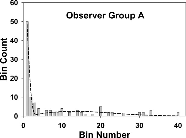
Table 1

Observed Number of Marks in the Different Bins, the Most Probable Number of Perceptual Hits and Misses, and the Expected Numbers of Perceptual Hits and Misses, for the Three Observer Groups

Observer Group Bin Index, i Observed Number of Marks Most Probable Expected Perceptual Hits, NHmax,i N

max

⁡

H Perceptual Misses, NMmax,i N

max

⁡

M Perceptual Hits, ⟨NHi⟩ 〈

〉 Perceptual Misses, ⟨NMi⟩ 〈

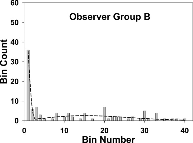
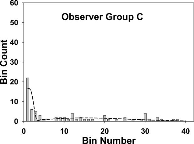
〉 A 1 50 50 0 48.3 0.163 2 10 10 0 11.8 0.487 3 7 0 7 0.090 0.802 4 4 0 4 0 1.102 5–40 42 0 42 0 49.9 B 1 36 36 0 35.4 0.146 2 6 6 0 6.26 0.437 3 7 0 7 0.0215 0.721 4 3 0 3 0 0.996 5–40 52 0 52 0 58.6 C 1 22 22 0 16.4 0.0964 2 6 6 0 13.7 0.288 3 5 4 1 1.69 0.475 4 3 0 3 0 0.828 5–40 37 0 37 0 37.8

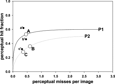
Group A represents the mammographers, group B the more experienced residents, and group C the less experienced residents. The sum of the perceptual hits and misses over all bins determines the perceptual operating points shown in Fig 7 . If the fourth bin is chosen as the acceptance criterion, the sum of the observed number of marks (column 3) for the first four bins determines the ordinate of the scored operating point , and the corresponding sum over the remaining bins determines the abscissa ( Fig 7 ).

Get Radiology Tree app to read full this article<

Table 2

Estimated Parameter Values, 95% Confidence Intervals (in Parentheses), and Goodness of Fit Statistics for the Three Groups of Observers

Observer Group Number of Marks N Model Parameters Goodness of Fit χ 2 /df/ P Value σ 1 σ 2 α A 113 0.14 (0.022) 3.2 (0.46) 0.53 (0.096) 15.0/6 /.02 B 104 0.13 (0.026) 3.7 (0.51) 0.40 (0.098) 15.0/8 /.06 C 73 0.21 (0.046) 3.7 (0.63) 0.44 (0.12) 19.8/5/.001

The fits are good for groups A and B and marginal for group C, as also seen visually in Fig 4, 5, and 6 . The σ 2 values (spread of the perceptual misses) are similar for all groups, group C had a marginally larger σ 1 value (spread of the perceptual misses), and group A had a marginally higher α value (probability that a mark is a perceptual hit). None of the differences was significant.

Get Radiology Tree app to read full this article<

$Figure 7, Shown are two perceptual FROC curves, labeled P1 and P2. The axes of a perceptual FROC plot are x: perceptual hit fraction and y: perceptual misses per images. The circles A, B, and C are perceptual FROC operating points corresponding to the three groups. The curves P1 and P2 are hypothetical perceptual FROC curves. These curves suggest that observer groups B and C are performing equivalently and that group A has superior performance. Note the difference in labeling of the axes in this figure as compared with Fig 1 . The filled circles in this plot, labeled a′, b′, and c′, are scored operating points, corresponding to the observer groups A, B, and C, respectively, that result if one chooses four bins (ie, 1°) as the acceptance angle. Note the upward-left shift toward (0, 1) of each scored point relative to the corresponding perceptual point (compare with Fig 1 “medium” → “large”), suggesting that this choice of acceptance angle will overestimate true performance.$

Get Radiology Tree app to read full this article<

Discussion

Get Radiology Tree app to read full this article<

Acknowledgments

Get Radiology Tree app to read full this article<

References

1. Egan J.P., Greenburg G.Z., Schulman A.I.: Operating characteristics, signal detectability and the method of free response. J Acoust Soc Am 1961; 33: pp. 993-1007.
2. Bunch P.C., Hamilton J.F., Sanderson G.K., et. al.: A free-response approach to the measurement and characterization of radiographic-observer performance. J Appl Photogr Eng 1978; 4: pp. 166-171.
3. Chakraborty D.P.: Maximum likelihood analysis of free-response receiver operating characteristic (FROC) data. Med Phys 1989; 16: pp. 561-568.
4. Chakraborty D.P., Breatnach E.S., Yester M.V., et. al.: Digital and conventional chest imaging: a modified ROC study of observer performance using simulated nodules. Radiology 1986; 158: pp. 35-39.
5. Chakraborty D.P., Winter L.H.L.: Free-response methodology: alternate analysis and a new observer-performance experiment. Radiology 1990; 174: pp. 873-881.
6. Chakraborty D.P., Berbaum K.S.: Observer studies involving detection and localization: modeling, analysis and validation. Med Phys 2004; 31: pp. 2313-2330.
7. Zheng B., Chakraborty D.P., Rockette H.E., et. al.: A comparison of two data analyses from two observer performance studies using jackknife ROC and JAFROC. Med Phys 2005; 32: pp. 1031-1034.
8. Penedo M., Souto M., Tahoces P.G., et. al.: Free-response receiver operating characteristic evaluation of lossy JPEG2000 and object-based set partitioning in hierarchical trees compression of digitized mammograms. Radiology 2005; 237: pp. 450-457.
9. Bornefalk H., Hermansson A.B.: On the comparison of FROC curves in mammography CAD systems. Med Phys 2005; 32: pp. 412-417.
10. Bornefalk H.: Estimation and comparison of CAD system performance in clinical settings. Acad Radiol 2005; 12: pp. 687-694.
11. Edwards D.C., Kupinski M.A., Metz C.E., et. al.: Maximum likelihood fitting of FROC curves under an initial-detection-and-candidate-analysis model. Med Phys 2002; 29: pp. 2861-2870.
12. Metz C.E.: Evaluation of digital mammography by ROC analysis.Doi K.Digital mammography ’96.1996.Elsevier ScienceAmsterdam, the Netherlands:pp. 61-68.
13. Metz C.E.: Some practical issues of experimental design and data analysis in radiological ROC studies. Investig Radiol 1989; 24: pp. 234-245.
14. Metz C.E.: ROC methodology in radiologic imaging. Investig Radiol 1986; 21: pp. 720-733.
15. Zheng B., Shah R., Wallace L., et. al.: Computer-aided detection in mammography: an assessment of performance on current and prior images. Acad Radiol 2002; 9: pp. 1245-1250.
16. Gur D., Stalder J.S., Hardesty L.A., et. al.: Computer-aided detection performance in mammographic examination of masses: assessment. Radiology 2004; 233: pp. 418-423.
17. Kallergi M., Carney G.M., Gaviria J.: Evaluating the performance of detection algorithms in digital mammography. Med Phys 1999; 26: pp. 267-275.
18. Giger M.L.Doi K.Giger M.L. et. al.Digital mammography ’96: current issues in CAD for mammography.1996.Elsevier Science B.V
19. Nishikawa R.M., Yarusso L.M.: Variations in measured performance of CAD schemes due to database composition and scoring protocol. Proc SPIE 1998; 3338: pp. 840-844.
20. Reiser I., Nishikawa R.M., Giger M.L., et. al.: Computerized mass detection for digital breast tomosynthesis directly from the projection images. Med Phys 2006; 33: pp. 482-491.
21. Sahiner B., Chan H.P., Hadjiiski L.M., et. al.: Joint two-view information for computerized detection of microcalcifications on mammograms. Med Phys 2006; 33: pp. 2574-2585.
22. Zheng B., Leader J.K., Abrams G.S., et. al.: A multi view based computer aided detection scheme for breast masses. Med Phys 2006; 33: pp. 3135-3143.
23. Duchowski A.T.: 2002.Clemson UniversityClemson, SC
24. Green D.M., Swets J.A.: 1966.John Wiley & SonsNew York
25. Metz C.E.: Basic principles of ROC analysis. Semin Nucl Med 1978; VIII: pp. 283-298.
26. Chakraborty D.P.: ROC curves predicted by a model of visual search. Phys Med Biol 2006; 51: pp. 3463-3482.
27. Chakraborty D.P.: A search model and figure of merit for observer data acquired according to the free-response paradigm. Phys Med Biol 2006; 51: pp. 3449-3462.
28. Kundel H.L., Nodine C.F.: A visual concept shapes image perception. Radiology 1983; 146: pp. 363-368.
29. Nodine C.F., Kundel H.L.: Using eye movements to study visual search and to improve tumor detection. RadioGraphics 1987; 7: pp. 1241-1250.
30. Kundel H.L., Nodine C.F.: Modeling visual search during mammogram viewing. Proc SPIE 2004; 5372: pp. 110-115.
31. Galassi M., Davies J., Theiler J., et. al.: 2005.Network Theory LimitedBristol, UK
32. Stuart A., Ord K., Arnold S.: Kendall’s advance theory of statistics: classical inference and the linear model2004.Oxford University PressNew York
33. Larsen R.J., Marx M.L.: 2001.Prentice-Hall IncUpper Saddle River, NJ
34. Press W.H., Flannery B.P., Teukolsky S.A., et. al.: 1988.Cambridge University PressCambridge, UK
35. Dorfman D.D., Alf E.: Maximum likelihood estimation of parameters of signal-detection theory and determination of confidence intervals—rating method data. J Math Psychol 1969; 6: pp. 487-496.
36. Mello-Thoms C., Dunn S., Nodine C.F., et. al.: The perception of breast cancers: a spatial frequency analysis of what differentiates missed from reported cancers. IEEE Trans Med Imaging 2003; 22: pp. 1297-1306.
37. Dorfman D.D., Berbaum K.S., Metz C.E.: ROC characteristic rating analysis: generalization to the population of readers and patients with the jackknife method. Investig Radiol 1992; 27: pp. 723-731.
38. Arora R., Kundel H.L., Beam C.A.: Perceptually based FROC analysis. Acad Radiol 2005; 12: pp. 1567-1574.

Spatial Localization Accuracy of Radiologists in Free-Response Studies Inferring Perceptual FROC Curves from Mark-Rating Data

Rationale and Objectives

Materials and Methods

Results

Conclusion

Materials and methods

Perceptual Hits and Misses

Rationale for the Spatial Distribution Model for the Marks

Mathematical Model for the Spatial Distribution of the Marks

Determination of the Parameters

Determination of the Most Probable Values of Perceptual Hits and Misses

Validity of the Model

Constructing Perceptual FROC Curves

Observer Study

Results

Discussion

Acknowledgments

References

Further Reading

Abstracts of Funded National Institutes of Health Grants

Acute Abdomen

Amaurosis Fugax Secondary to Imaging Methods of MRI Scan