
Rationale and Objectives
The identification of body fluids in computed tomography poses a major diagnostic challenge. The chemical composition of body fluids deviates only slightly from water with very similar computed tomographic (CT) values, which typically range from 0 to 100 HU. The aim of this study was to assess physical and chemical properties of different body fluids in an ex vivo setting.
Materials and Methods
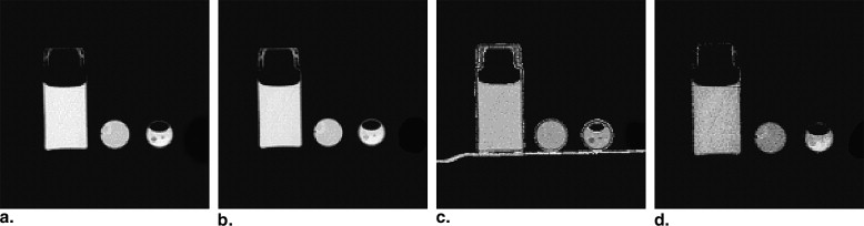
A total of 44 samples of blood, blood mixed with pus, pus, bile, and urine obtained during diagnostic and therapeutic punctures were scanned at 80 and 140 kV. Data was quantitatively assessed using the spectral ρZ -projection algorithm, which converts dual-energy CT scans into mass density ( ρ ) and effective atomic number ( Z eff. ) information.
Results
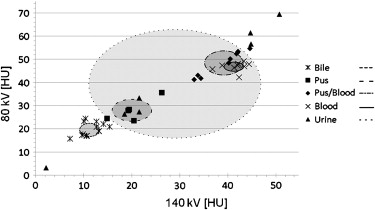
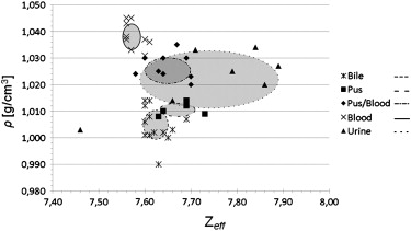
Attenuation values measured at 80 and 140 kV were largely overlapping. CT values allowed, to some degree, for the differentiation of bile or pus from blood or the blood/pus mixture. By applying the ρZ -projection, most substances, except for urine, were distinguishable with only small standard deviations ranging between 0.003 and 0.007 g/cm 3 for mass density and between 0.020 and 0.043 for Z eff. .
Conclusion
The ρZ -projection method is suited to quantitatively assess mass density and effective atomic number of ex vivo body fluid samples. In clinical routine, this technique might be useful for identifying unclear fluid collections even in unenhanced computed tomography.
Computed tomography is one of the most important non-invasive diagnostic imaging modalities. It provides three-dimensional representations of the x-ray attenuation coefficient μ (r) with submillimeter spatial resolution. However, it is limited in soft tissue contrast resolution . Various types of soft tissue and lesions differ only slightly in density and chemical composition and thus their measured x-ray attenuation coefficients are very similar.
To overcome this limitation, intravenous contrast agents are routinely administered. However, differentiation of nonperfused fluid collections such as hematoma, lymphoceles, abscess, or urinoma remains difficult , particularly if there are ambiguous clinical findings, or shortly after surgery. Moreover, there are many patients who may not receive iodinated contrast agents. Over the last decade, several studies have addressed the problem of fluid differentiation in computed tomography, but failed to provide clinically applicable solutions . Thus, low contrast resolution of noncontrast enhanced computed tomography is still a relevant issue in fluid differentiation.
Get Radiology Tree app to read full this article<
Get Radiology Tree app to read full this article<
Material and methods
Get Radiology Tree app to read full this article<
Get Radiology Tree app to read full this article<
Get Radiology Tree app to read full this article<
Get Radiology Tree app to read full this article<
Get Radiology Tree app to read full this article<
Get Radiology Tree app to read full this article<
Get Radiology Tree app to read full this article<
Get Radiology Tree app to read full this article<
Results
Get Radiology Tree app to read full this article<
Get Radiology Tree app to read full this article<
Get Radiology Tree app to read full this article<
Get Radiology Tree app to read full this article<
Table 1
Summary of the Attenuation Values at Different Tube Voltages, Mass Densities, and Effective Atomic Numbers as Computed using the ρZ -algorithm. Except for Pus and Bile, Attenuation Values are Widely Overlapping, Limiting Fluid Differentiation
80 kV [HU] 140 kV [HU] Mass Density [ ρ ; g/cm 3 ] Eff. Atomic Number [ Z eff. ] Blood (n = 9) 46.8 ± 2.0 (42.2–49.2) 41.6 ± 2.4 (36.8–44.4) 1.038 ± 0.005 (1.031–1.045) 7.577 ± 0.020 (7.560–7.610) Blood + Pus (n = 9) 48.7 ± 5.3 (41.3–54.6) 39.2 ± 4.3 (33.0–44.6) 1.027 ± 0.005 (1.020–1.035) 7.636 ± 0.043 (7.580–7.700) Pus (n = 5) 27.9 ± 4.8 (23.5–35.6) 20.1 ± 4.1 (14.9–26.3) 1.011 ± 0.003 (1.008–1.014) 7.676 ± 0.041 (7.630–7.730) Bile (n = 13) 20.0 ± 3.1 (15.8–24.4) 11.9 ± 2.7 (7.2–15.4) 1.005 ± 0.007 (0.990–1.014) 7.625 ± 0.028 (7.600–7.690) Urine (n = 7) 39.7 ± 3.6 (3.2–69.4) 29.2 ± 17.8 (2.2–50.7) 1.022 ± 0.011 (1.003–1.034) 7.744 ± 0.149 (7.460–7.890)
Data are given as Mean ± Standard Deviation. Values in Brackets Indicate Minimum and Maximum.
Get Radiology Tree app to read full this article<
Get Radiology Tree app to read full this article<
Table 2
The Means of the Five Categories of Fluids were Compared for the Attenuation Values at 80 and 140 kV, Mass Density, and Effective Atomic Number with t -tests. Applying the ρZ Projection Method, Blood becomes Distinguishable from Mixtures of Blood and Pus with ρ and Z eff. being Significantly Different for each Fluid. For the other Categories of Fluids, there are No Major Differences Comparing the Attenuation Values with the Results of the ρZ Projection Method
Parameter Blood + Pus Pus Bile Urine Blood 80 kV_P_ = .3293P < .0001P < .0001P = .3795 140 kV_P_ = .1631P < .0001P < .0001P = .0557 ρ_P_ = .0003P < .0001P <.0001P = .0016Z eff.__P = .0018P < .0001P = .0003P = .0047 Blood + Pus 80 kV -P < .0001P < .0001P = .2820 140 kV -P < .0001P < .0001P = .1232 ρ -P < .0001P < .0001P = .2426Z eff. -P = .1161P = .4743P = .0559 Pus 80 kV - -P = .0007P = .3023 140 kV - -P < .0001P = .2939 ρ - -P = .0866P =.0569Z eff. - -P =.0076P = .3494 Bile 80 kV - - -P = .0072 140 kV - - -P = .0025 ρ - - -P = .0005Z eff. - - -P = .0106
Get Radiology Tree app to read full this article<
Discussion
Get Radiology Tree app to read full this article<
Get Radiology Tree app to read full this article<
Get Radiology Tree app to read full this article<
Get Radiology Tree app to read full this article<
Get Radiology Tree app to read full this article<
Get Radiology Tree app to read full this article<
Get Radiology Tree app to read full this article<
Get Radiology Tree app to read full this article<
Conclusion
Get Radiology Tree app to read full this article<
Appendix
Get Radiology Tree app to read full this article<
Get Radiology Tree app to read full this article<
(μ1μ2)=ρ⋅⎛⎝⎜∫w1(E)(κρ)(E,Z)dE∫w2(E)(κρ)(E,Z)dE⎞⎠⎟=ρ(f1(Z)f2(Z)). (
μ
1
μ
2
)
=
ρ
⋅
(
∫
w
1
(
E
)
(
κ
ρ
)
(
E
,
Z
)
d
E
∫
w
2
(
E
)
(
κ
ρ
)
(
E
,
Z
)
d
E
)
=
ρ
(
f
1
(
Z
)
f
2
(
Z
)
)
.
Here the spectral attenuation coefficient ( κ/ρ ) is factorized into the mass density ρ and the specific spectral attenuation function ( κ/ρ )(E). Note that the left side of ( Eqn 1 ) contains the measured values
μi=(1+Hi1000)μH2O μ
i
=
(
1
+
H
i
1000
)
μ
H
2
O
and the right side can be calculated for the known spectral weighting functions w i ( E ) and elemental atomic basis functions ( κ/ρ )( E ).
Get Radiology Tree app to read full this article<
Get Radiology Tree app to read full this article<
(μ1(ρ,Z)μ2(ρ,Z))→(ρ(μ1,μ2)Z(μ1,μ2)). (
μ
1
(
ρ
,
Z
)
μ
2
(
ρ
,
Z
)
)
→
(
ρ
(
μ
1
,
μ
2
)
Z
(
μ
1
,
μ
2
)
)
.
As the numerical solution
Z=F−1(μ1μ2),ρ=μ1f1(Z)=μ1f1(F−1(μ1μ2)) Z
=
F
-
1
(
μ
1
μ
2
)
,
ρ
=
μ
1
f
1
(
Z
)
=
μ
1
f
1
(
F
−
1
(
μ
1
μ
2
)
)
is obtained with
fi(Z)=∫wi(E)(κρ)(E,Z)dE,F(Z)=f1(Z)f2(Z). f
i
(
Z
)
=
∫
w
i
(
E
)
(
κ
ρ
)
(
E
,
Z
)
dE
,
F
(
Z
)
=
f
1
(
Z
)
f
2
(
Z
)
.
The functions f 1 (Z), f 2 (Z) and F ( Z ) can be calculated prior to the measurement with the known spectral weighting functions w i ( E ) and tabulated ( κ/ρ )( E, Z ) from experimental data by, e.g., Perkins et al and Cullen et al . Equations (3a, b) directly transform two measured images into ρ and Z images. For medical computed tomography we can generally expect Z eff. to be lying in the interval [1… 20] and ρ in the interval [0… 2] g/cm 3 .
Get Radiology Tree app to read full this article<
Get Radiology Tree app to read full this article<
μ=∑nk=1ρk∫w(E)(κρ)(E,Zk)dE. μ
=
∑
k
=
1
n
ρ
k
∫
w
(
E
)
(
κ
ρ
)
(
E
,
Z
k
)
d
E
.
For a known stoichiometric composition of a compound material the associated Z eff. can be calculated.
Get Radiology Tree app to read full this article<
Get Radiology Tree app to read full this article<
Get Radiology Tree app to read full this article<
References
1. Filly R.A., Sommer F.G., Minton M.J.: Characterization of biological fluids by ultrasound and computed tomography. Radiology 1980; 134: pp. 167-171.
2. Gupta S., Seith A., Sud K., et. al.: CT in the evaluation of complicated autosomal dominant polycystic kidney disease. Acta Radiol 2000; 41: pp. 280-284.
3. Nandalur K.R., Hardie A.H., Bollampally S.R., et. al.: Accuracy of computed tomography attenuation values in the characterization of pleural fluid: an ROC study. Acad Radiol 2005; 12: pp. 987-991.
4. Alvarez R.E., Macovski A.: Energy-selective reconstructions in X-ray computerized tomography. Phys Med Biol 1976; 21: pp. 733-744.
5. Macovski A., Alvarez R.E., Chan J.L., et. al.: Energy dependent reconstruction in X-ray computerized tomography. Comput Biol Med 1976; 6: pp. 325-336.
6. Heismann B.J., Leppert J., Stierstorfer K.: Density and atomic number measurements with spectral x-ray attenuation method. J Appl Phys 2003; 94: pp. 2073-2079.
7. Stonestrom J.P., Alvarez R.E., Macovski A.: A framework for spectral artifact corrections in x-ray CT. IEEE Trans Biomed Eng 1981; 28: pp. 128-141.
8. Weaver J.B., Huddleston A.L.: Attenuation coefficients of body tissues using principal-components analysis. Med Phys 1985; 12: pp. 40-45.
9. Vetter J.R., Holden J.E.: Correction for scattered radiation and other background signals in dual-energy computed tomography material thickness measurements. Med Phys 1988; 15: pp. 726-731.
10. Avrin D.E., Macovski A., Zatz L.E.: Clinical application of Compton and photo-electric reconstruction in computed tomography: preliminary results. Invest Radiol 1978; 13: pp. 217-222.
11. Kalender W.A., Perman W.H., Vetter J.R., et. al.: Evaluation of a prototype dual-energy computed tomographic apparatus. I. Phantom studies. Med Phys 1986; 13: pp. 334-339.
12. Heismann B.J.: Atomic number measurement precision of spectral decomposition methods for CT. IEEE Nuclear Science Symposium Conference Record 2005; 5: pp. 2741-2742.
13. International Commission on Radiation Units and Measurements (ICRU): Photon, electron, proton and neutron interaction data for body tissues (Report 46).1992.ICRUBethesda, MD
14. Johnson T.R., Krauss B., Sedlmair M., et. al.: Material differentiation by dual energy CT: initial experience. Eur Radiol 2007; 17: pp. 1510-1517.
15. Pontana F., Faivre J.B., Remy-Jardin M., et. al.: Lung perfusion with dual-energy multidetector-row CT (MDCT): feasibility for the evaluation of acute pulmonary embolism in 117 consecutive patients. Acad Radiol 2008; 15: pp. 1494-1504.
16. Primak A.N., Fletcher J.G., Vrtiska T.J., et. al.: Noninvasive differentiation of uric acid versus non-uric acid kidney stones using dual-energy CT. Acad Radiol 2007; 14: pp. 1441-1447.
17. Perkins ST, Cullen DE, Chen MH, et al. Tables and graphs of atomic subshell and relaxation data derived from the LLNL evaluated atomic data library (EADL), Z = 1-100. Lawrence Livermore National Laboratory Report UCRL-50400, Vol. 30. Livermore, CA, 1991.
18. Cullen DE, Chen MH, Hubbell JH, et al. Tables and graphs of photon-interaction cross-sections from 10 eV to 100 GeV derived from the LLNL evaluated photon data library. Lawrence Livermore National Laboratory Report UCRL-50400, Vol. 6. Livermore, CA, 1989.