
A major initiative of the Quantitative Imaging Biomarker Alliance is to develop standards-based documents called “Profiles,” which describe one or more technical performance claims for a given imaging modality. The term “actor” denotes any entity (device, software, or person) whose performance must meet certain specifications for the claim to be met. The objective of this paper is to present the statistical issues in testing actors’ conformance with the specifications. In particular, we present the general rationale and interpretation of the claims, the minimum requirements for testing whether an actor achieves the performance requirements, the study designs used for testing conformity, and the statistical analysis plan. We use three examples to illustrate the process: apparent diffusion coefficient in solid tumors measured by MRI, change in Perc 15 as a biomarker for the progression of emphysema, and percent change in solid tumor volume by computed tomography as a biomarker for lung cancer progression.
Introduction
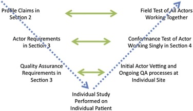
The Quantitative Imaging Biomarker Alliance (QIBA) initiative is to advance quantitative imaging and the use of quantitative imaging biomarkers (QIBs) both in clinical trials and in clinical practice . One effort in this initiative is to develop standards-based quantitative imaging documents called “Profiles.” These Profiles describe the (1) clinical context for the biomarker, (2) one or more technical performance claims for a given imaging modality (e.g. precision of the measurement for computed tomography (CT), magnetic resonance imaging (MRI), positron emission tomography, or ultrasound), (3) a list of actors including hardware and software that play defined roles in meeting the claims, (4) technical and performance requirements for each of those actors organized by activities they perform for achieving the claims, (5) summaries of the groundwork scientific studies that support the technical performance claims, and (6) procedures for testing conformity to the technical and performance requirements or an overarching claim. The term “actor” is used in QIBA Profiles to denote any entity (device, software, person, or site) whose performance must meet certain specifications for the claim to be met.
Through a large volunteer effort, two workshops sponsored by QIBA were conducted to develop standard statistical methods for defining technical performance metrics for QIBs . These statistical methods provide the framework for comparing technical performances of imaging procedures in the groundwork studies and for characterizing the performance in the Profile claims.
The objective of this paper is to present the statistical issues in testing conformance to the performance requirements in the QIBA Profiles. In particular, we present the general rationale and interpretation of the claims, the minimum requirements for testing whether an actor achieves the performance requirements, the study designs used for testing conformity, and the statistical analysis plan for the test. We use three examples to illustrate the process:
1. Apparent diffusion coefficient (ADC) in solid tumors measured by MRI to gain insight into the microstructural composition of a tumor,
2. Change in Perc 15 (the 15th percentile of the attenuation curve as measured by CT) as a biomarker for the progression of emphysema, and
Get Radiology Tree app to read full this article<
Get Radiology Tree app to read full this article<
QIBA’s Performance Claims
Understanding the Claim Statements
Get Radiology Tree app to read full this article<
Get Radiology Tree app to read full this article<
Get Radiology Tree app to read full this article<
Get Radiology Tree app to read full this article<
Get Radiology Tree app to read full this article<
Determining Appropriate Values to Use in the Claim Statements
Get Radiology Tree app to read full this article<
Get Radiology Tree app to read full this article<
TABLE 1
Guidelines for Choosing Values for Claim Statements
Step Description 1 Choose statistical metric for performance 2 Determine patient and/or tumor characteristics that can degrade performance for the quantitative imaging biomarker 3 Identify plausible set of values for performance 4 Consider clinical requirements for performance 5 Consider the sample size requirements for actors to test their imaging procedure against the claim value 6 Choose the performance value from the plausible set of values in step 3, taking into consideration steps 4–5.
Get Radiology Tree app to read full this article<
Step 1: Choose Metric
Get Radiology Tree app to read full this article<
TABLE 2
Statistical Metrics Used in the Claim Statements
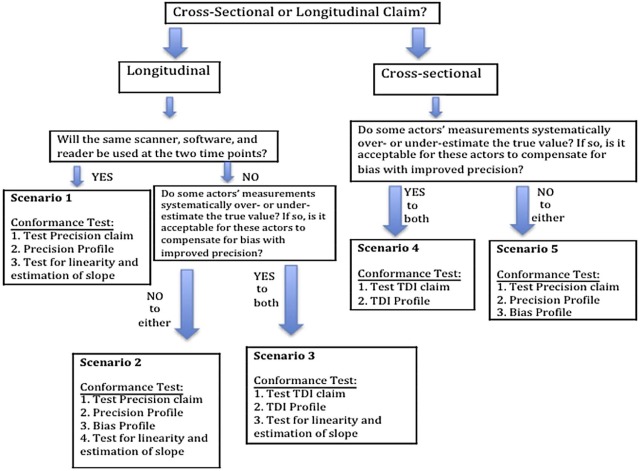
Example Rationale Statistical Metric Interpretation ADC in solid tumors Cross-sectional claim with negligible bias Within-subject (or within-tumor) standard deviation (wSD) × (95% confidence factor) The variability seen in multiple measurements on a subject when no biologic change has occurred and the same imaging procedures are used for all measurements. Change in Perc 15 for monitoring emphysema Longitudinal claim;
Same imaging procedures at two time points WRepeatability
coefficient (RC) The difference between any two measurements on a case is expected to fall between −RC and +RC for 95% of replicated measurements. It represents the minimum detectable difference, with 95% confidence. % Change in CT tumor volume Longitudinal claim;
Different imaging procedures at two time points Reproducibility coefficient (RDC) is used in the claim statement. The total deviation index with 95% coverage for change (TDI 95% ) is used for testing conformance. The RDC is a measure of precision that is used when imaging procedures differ at the two time points. It has a similar interpretation as the RC: it is the minimum detectable difference, with 95% confidence. Because it can be measured directly from clinical studies, it is used in the claim statement. When testing conformance, the bias of the imaging procedures at the two time points will likely differ and this must be accounted for. Thus, the TDI is used for conformance testing. It includes components of both precision and bias. Of the differences between the measurements and their true value, 95% is <TDI 95% . The TDI cannot be measured directly; rather, an actor’s bias and precision are estimated in separate studies. See section on Trade-off between Precision and Bias
Get Radiology Tree app to read full this article<
Step 2: Determine Characteristics Which Degrade Precision
Get Radiology Tree app to read full this article<
Step 3: Identify Plausible Set of Values
Get Radiology Tree app to read full this article<
Get Radiology Tree app to read full this article<
Step 4: Consider Clinical Requirements
Get Radiology Tree app to read full this article<
Step 5: Consider Sample Size for Conformance Test
Get Radiology Tree app to read full this article<
Ho:theactor’sperformanceisworsethantherequirementvs.HA:theactor’sperformanceisatleastasgoodastherequirement H
o
:
t
h
e
actor
’
s
performance
i
s
worse
than
t
h
e
requirement
vs
.
H
A
:
t
h
e
actor
’
s
performance
i
s
a
t
least
a
s
good
a
s
t
h
e
requirement
Get Radiology Tree app to read full this article<
Get Radiology Tree app to read full this article<
TABLE 3
Sample Size for Test of Precision Using Repeatability Coefficient
(θ/δ) 2 # Cases Needed 0.1 4 0.2 7 0.3 11 0.4 17 0.5 29 0.6 51 0.7 102 0.8 256
Get Radiology Tree app to read full this article<
Step 6: Choose Performance Value
Get Radiology Tree app to read full this article<
Minimum Conformance Requirements
Get Radiology Tree app to read full this article<
Get Radiology Tree app to read full this article<
Get Radiology Tree app to read full this article<
Get Radiology Tree app to read full this article<
Get Radiology Tree app to read full this article<
Get Radiology Tree app to read full this article<
Get Radiology Tree app to read full this article<
Get Radiology Tree app to read full this article<
Get Radiology Tree app to read full this article<
Get Radiology Tree app to read full this article<
Testing Conformity
Get Radiology Tree app to read full this article<
Steps in Testing Conformity
Get Radiology Tree app to read full this article<
TABLE 4
Testing Precision Using CT Volumetry for Illustration \*
Step Description 1. Make measurements on N cases For each case, measure the tumor volume at time point 1 (denoted Y i1 ) and at time point 2 (Y i2 ) where i denotes the i -th case ( i = 1, 2, … N ). 2. For each case, calculate mean and wSD 2 For each case, calculate the mean and within-tumor SD: Y¯¯¯i=(Yi1+Yi2)/2 Y
¯
i
=
(
Y
i
1
+
Y
i
2
)
/
2 and wSD2i=(Yi1−Yi2)2/2 w
S
D
i
2
=
(
Y
i
1
−
Y
i
2
)
2
/
2 . (Note that some authors suggest a correction to this wSD estimate or a model-based estimate to account for the small number of replicate measurements.) 3. Estimate wSD or wCV From the N cases, estimate within-tumor SD (wSD) or CV (wCV):
wSD=∑Ni=1wSD2i/N−−−−−−−−−−−−√ w
S
D
=
∑
i
=
1
N
w
S
D
i
2
/
N and wCV=∑Ni=1(wSD2i/Y¯¯¯2i)/N−−−−−−−−−−−−−−−−−−√ w
C
V
=
∑
i
=
1
N
(
w
S
D
i
2
/
Y
¯
i
2
)
/
N .
(Note that averaging over the N cases is appropriate when we can assume that the wSD is constant over the range of tumor volume values.) 4. Estimate RC or %RC \* Estimate the repeatability coefficient (RC) or %RC:
RCˆ=2.77×wSD R
C
=
2.77
×
w
S
D and %RCˆ=2.77×wCV×100 %
R
C
=
2.77
×
w
C
V
×
100 . For the CT volumetry example, %RC is used. 5. Calculate test statistic and assess compliance The null hypothesis is that the RC does not satisfy the requirement in the Profile (i.e. the RC is too large); the alternative hypothesis is that the RC does satisfy the requirement. The test statistic T is: T=N×(%RCˆ2)δ2 T
=
N
×
(
%
R
C
2
)
δ
2 , where δ δ is the performance value from the Profile claim statement (i.e. δ=40% δ
=
40
% ). Compliance with the claim is shown if T<χ2α,N T
<
χ
α
,
N
2 , where χ2α,N χ
α
,
N
2 is the α-th percentile of a chi square distribution † with N degrees of freedom (for a one-sided test with α type I error rate). 6. Construct precision profile Estimate %RC as a function of tumor size and check that all %RC≤δ %
RC
≤
δ ?.
CI, confidence interval; RC, repeatability coefficient; SD, standard deviation; wCV, within-tumor coefficient of variation; wSD, within-tumor standard deviation.
Get Radiology Tree app to read full this article<
Get Radiology Tree app to read full this article<
TABLE 5
Testing Bias and Linearity using CT Volumetry for Illustration \*
Step Description 7: Make measurements from N cases For each case calculate the tumor volume (denoted Y i ), where i denotes the i -th case ( i = 1, 2, … N ). 8. Calculate individual bias For each case calculate the bias or % bias:
bi=(Yi−Xi) b
i
=
(
Y
i
−
X
i
) and %bi=[(Yi−Xi)/Xi]×100 %
b
i
=
[
(
Y
i
−
X
i
)
/
X
i
]
×
100 , where X i is the measurand value (i.e. true value). For CT volumetry, % b is used. 9. Estimate overall bias and its variance \* Over N cases, estimate the bias: bˆ=∑Ni=1%bi/N b
=
∑
i
=
1
N
%
b
i
/
N . The estimate of the variance of the bias (i.e. between-case variance) is Varˆb=∑Ni=1(%bi−bˆ)2/(N−1) V
a
r
b
=
∑
i
=
1
N
(
%
b
i
−
b
)
2
/
(
N
−
1
) . 10. Construct 95% CI for bˆ b
The 95% CI for the bias is bˆ±tα=0.025,(N−1)df×Varˆb−−−−√ b
±
t
α
=
0.025
,
(
N
−
1
)
d
f
×
V
a
r
b , where tα=0.025,(N−1)df t
α
=
0.025
,
(
N
−
1
)
d
f is from the Student t distribution † with α = 0.025 and ( N − 1) degrees of freedom. To test whether the actor’s bias satisfies the performance requirement in the Profile, the smallest and largest values in the 95% CI are examined. If the smallest value is greater than the minimum requirement stated in the Profile and the largest value is less than the maximum requirement stated in the Profile, then the performance requirement for the overall bias is met. 11. Bias Profile Separate the cases into strata based on covariates known to affect bias (tumor size and density). For each stratum, estimate the bias. 12. Perform OLS regression Fit an ordinary least squares (OLS) regression of the Y i s on X i s. A quadratic term is first included in the model to rule out nonlinear relationships: Y=βo+β1X+β2X2 Y
=
β
o
+
β
1
X
+
β
2
X
2 . Then a linear model should be fit: Y=βo+β1X Y
=
β
o
+
β
1
X where R-squared (R 2 ) > 0.90. 13. Construct 95% CI for slope Let β1ˆ β
1
denote the estimated slope from step 12 (assuming β2=0 β
2
=
0 ). Calculate its variance as Varˆβ1={∑Ni=1(Yi−Yˆi)2/(N−2)}/∑Ni=1(Xi−X¯¯¯)2 V
a
r
β
1
=
{
∑
i
=
1
N
(
Y
i
−
Y
i
)
2
/
(
N
−
2
)
}
/
∑
i
=
1
N
(
X
i
−
X
¯
)
2 , where Yˆi Y
i is the fitted value of Y i from the regression line and X¯¯¯ X
¯ is the mean of the true values. The 95% CI is β1ˆ±tα=0.025,(N−2)dfVarˆβ1−−−−−√ β
1
±
t
α
=
0.025
,
(
N
−
2
)
d
f
V
a
r
β
1
CI, confidence interval; OLS, ordinary least squares.
Get Radiology Tree app to read full this article<
Get Radiology Tree app to read full this article<
Get Radiology Tree app to read full this article<
Precision
Get Radiology Tree app to read full this article<
Ho:θ>δversusHA:θ≤δ H
o
:
θ
δ
versus
H
A
:
θ
≤
δ
where θ is the actor’s precision (e.g. the actor’s RC, where larger values indicate worse precision) and δ is the precision value from the claim statement. This is a one-sided test, i.e. under the null hypothesis, the actor’s precision is considered inferior to the Profile claim. If the null hypothesis is rejected, then we conclude that the actor’s precision is at least as good as the performance in the claim statement (alternative hypothesis).
Get Radiology Tree app to read full this article<
Get Radiology Tree app to read full this article<
Get Radiology Tree app to read full this article<
Bias
Get Radiology Tree app to read full this article<
Get Radiology Tree app to read full this article<
Linearity
Get Radiology Tree app to read full this article<
Get Radiology Tree app to read full this article<
Get Radiology Tree app to read full this article<
Get Radiology Tree app to read full this article<
Get Radiology Tree app to read full this article<
Trade-off between Precision and Bias
Get Radiology Tree app to read full this article<
TDI95%ˆ=Φ−1(1−1−0.952)|εˆ| T
D
I
95
%
=
Φ
−
1
(
1
−
1
−
0.95
2
)
|
ε
|
where Φ−1 Φ
−
1 is the inverse cumulative normal distribution (i.e. 1.96 for 95% coverage) and εˆ ε
is the estimate of the root mean square deviation:
MSDˆ=εˆ2=(bias)2+s2Y, M
S
D
=
ε
2
=
(
bias
)
2
+
s
Y
2
,
where bias is an estimate of the bias of the measurements (from step 9 in Table 5 ) and s2Y s
Y
2 is an estimate of the within-subject (e.g. within-tumor) variance (from step 3 in Table 4 ).
Get Radiology Tree app to read full this article<
Get Radiology Tree app to read full this article<
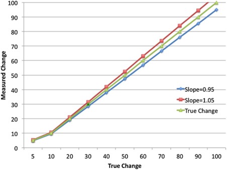
![Figure 4, Illustration of the trade-off between Precision (expressed as the repeatability coefficient [RC]) and Bias for constant total deviation index with 95% coverage (TDI 95% ) of 40%.](https://storage.googleapis.com/dl.dentistrykey.com/clinical/StatisticalIssuesinTestingConformancewiththeQuantitativeImagingBiomarkerAllianceQIBAProfileClaims/3_1s20S1076633216000544.jpg)
Get Radiology Tree app to read full this article<
Sample Size Requirements for Testing Conformity
Get Radiology Tree app to read full this article<
Ho:θ>δversusHA:θ≤δ H
o
:
θ
δ
versus
H
A
:
θ
≤
δ
where θ is the actor’s precision and δ is the precision value from the claim statement. To compute sample size for a study to test this set of hypotheses, the following must be specified:
Get Radiology Tree app to read full this article<
Get Radiology Tree app to read full this article<
Get Radiology Tree app to read full this article<
Get Radiology Tree app to read full this article<
Get Radiology Tree app to read full this article<
TABLE 6
Sample Size for Evaluating Bias
Half-width of 95% Confidence Interval for Bias ±1% ±2% ±3% ±4% ±5% Var b \* = 5% 22 8 ≤5 ≤5 ≤5 Var b = 10% 42 13 7 ≤5 ≤5 Var b = 15% 61 17 9 7 ≤5 Var b = 20% 80 22 12 8 6 Var b = 25% 99 27 14 9 7
Get Radiology Tree app to read full this article<
Get Radiology Tree app to read full this article<
Discussion
Get Radiology Tree app to read full this article<
Get Radiology Tree app to read full this article<
Get Radiology Tree app to read full this article<
Get Radiology Tree app to read full this article<
Get Radiology Tree app to read full this article<
Acknowledgement
Get Radiology Tree app to read full this article<
References
1. Buckler A.J., Bresolin L., Dunnick N.R., et. al.: A collaborative enterprise for multi-stakeholder participation in the advancement of quantitative imaging. Radiology 2011; 258: pp. 906-914.
2. Kessler L.G., Barnhart H.X., Buckler A.J., et. al.: The emerging science of quantitative imaging biomarkers: terminology and definitions for scientific studies and for regulatory submissions. Stat Methods Med Res 2015; 24: pp. 9-26.
3. Raunig D., McShane L.M., Pennello G., et. al.: Quantitative imaging biomarkers: a review of statistical methods for technical performance assessment. Stat Methods Med Res 2015; 24: pp. 27-67.
4. Obuchowski N.A., Reeves A.P., Huang E.P., et. al.: Quantitative Imaging biomarkers: a review of statistical methods for computer algorithm comparisons. Stat Methods Med Res 2015; 24: pp. 68-106.
5. Obuchowski N.A., Barnhart H.X., Buckler A.J., et. al.: Statistical issues in the comparison of quantitative imaging biomarker algorithms using pulmonary nodule volume as an example. Stat Methods Med Res 2015; 24: pp. 107-140.
6. Huang E.P., Wang X.-F., Roy Choudhury K., et. al.: Meta-analysis of the technical performance of an imaging assay: guidelines and statistical methodology. Stat Methods Med Res 2015; 24: pp. 141-174.
7. Available at: https://www.rsna.org/QIBA
8. Reeves A.P., Jirapatnakul A.C., Biancardi A.M., et. al.: The VOLCANO’09 challenge: preliminary results.Second international workshop of pulmonary image analysis.2009.pp. 353-364.
9. Bolch B.W.: More on unbiased estimation of the standard deviation. Am Stat 1968; 22: pp. 27.
10. Ashton E., Raunig D., Ng C., et. al.: Scan-rescan variability in perfusion assessment of tumors in MRI using both model and data-derived arterial input functions. J Magn Reson Imaging 2008; 28: pp. 791-796.
11. Petrick N., Kim H.J.G., Clunie D., et. al.: Comparison of 1D, 2D, and 3D nodule sizing methods by radiologists for spherical and complex nodules on thoracic CT phantom images. Acad Radiol 2014; 21: pp. 30-40.
12. Stolk J., Putter H., Bakker M.E., et. al.: Progression parameters for emphysema: a clinical investigation. Respir Med 2007; 101: pp. 1924-1930.
13. Dixon W.J., Massey F.J.: Introduction to statistical analysis.4th ed.1983.McGraw-HillNew York
14. Barnhart H.X., Barboriak D.P.: Applications of the repeatability of quantitative imaging biomarkers: a review of statistical analysis of repeat data sets. Transl Oncol 2009; 2: pp. 231-235.