Statistical Power Considerations for a Utility Endpoint in Observer Performance Studie s

Rationale and Objectives

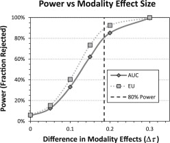
The purpose of this investigation is to compare the statistical power of the most common measure of performance for observer performance studies, area under the ROC curve (AUC), to an expected utility (EU) endpoint.

Materials and Methods

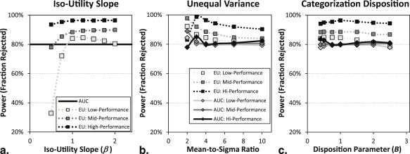
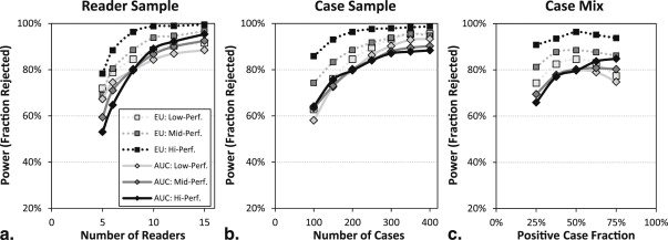
We have modified a well-known simulation procedure developed by Roe and Metz for statistical power analysis in receiver operating characteristic (ROC) studies. Starting from a set of baseline simulations, we investigate the effects of three parameters that describe properties of the observers (iso-utility slope, unequal variance, and tendency to favor more aggressive or conservative actions) and three parameters that affect experimental design (number of readers, number of cases, and fraction of positive cases).

Results

The EU endpoint generally has good statistical power relative to AUC in our simulations. Of 396 total conditions simulated, EU had higher statistical power in 377 cases (95%). In 246 of these cases, EU power was 5 percentage points or more higher than AUC. In simulation runs evaluating the effect of the number of readers and cases on the baseline simulations, EU measure had equivalent power to AUC with fewer readers (9% to 28%) or fewer cases (18% to 41%).

Conclusion

These simulation studies provide further motivation for considering EU in studies of screening mammography technology and they motivate investigations of utility in other diagnostic tasks.

Decisions have consequences. This truism is particularly applicable to medical decisions that affect the health and well-being of patients as well as the financial cost of care to payers. In this context, diagnostic medical imaging technology can be categorized as providing support for medical decision-making. It is widely recognized that the evaluation of diagnostic medical imaging technology should represent its effect on decision-making performance in addition to physical measurements of fundamental imaging characteristics (noise, resolution, contrast). The medical imaging community generally expects that proponents of new techniques will use some measure of observer performance as an endpoint of validation studies. For example, the United States Food and Drug Administration routinely asks manufacturers of medical imaging technology to provide reasonable assurance that a device is effective through observer performance metrics .

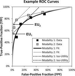
In many cases of interest, technology can be assessed in the framework of a binary task. In such cases, receiver operating characteristic (ROC) analysis is a well-established method to characterize the effect of technology on diagnostic ability . The ROC curve plots the tradeoff between the true-positive fraction (TPF also referred to as sensitivity) and the false positive fraction (FPF, also 1 - Specificity). However, to be useful for quantitative comparisons, a summary value must be extracted from the ROC curve as a figure of merit indicating the level of performance. In the field of medical imaging, that number has most commonly been the area under the ROC curve (AUC) . AUC has an intuitive interpretation as the average sensitivity over all possible specificities as well as the probability that a randomly chosen example from the population with disease will be detected over a randomly chosen example from the normal (nondiseased) population . But AUC does not account for the prevalence of disease or the consequences of decisions, which both factor heavily in clinical decisions.

Get Radiology Tree app to read full this article<

Materials and methods

A Roe and Metz Type Simulation

Get Radiology Tree app to read full this article<

AUC and Utility Endpoints

Get Radiology Tree app to read full this article<

EU=Max(FPF,TPF)∈ROC(TPF−βFPF), EU

Max

(

)

∈

(

TPF

−

FPF

)

where (FPF,TPF)∈ROC (

FPF

TPF

)

∈

ROC indicates all points on the ROC curve. The quantity, TPF− β FPF, can be thought of as the y intercept of a line with slope β that passes through the point (FPF, TPF). It can also be considered a FPF “corrected” sensitivity, where β scales the penalty associated with the given false-positive rate. In either case, the figure of merit consists of maximizing this value over all possible points on the ROC curve. Because the maximal value is found when the line is tangent to a smooth ROC curve, β is often referred to as the ROC slope. Utility theory suggests that this value should be determined by the four possible outcome utilities and by the prevalence of disease. In this case, lines of slope β may be considered iso-utility lines, and the y intercept can be related to the total utility of the decision process. Figure 1 shows graphically how EU endpoints are derived from hypothetical ROC data.

Get Radiology Tree app to read full this article<

Scope of Studies

Get Radiology Tree app to read full this article<

Table 1

Default Simulation Parameters

Effect Label or Parameter Default Roe and Metz variance structure LL, LH, HL, and HH See reference Level of performance Low, mid, and high AUC = 0.70, 0.86, or 0.96 Iso-utility slope_β_ 1.03 ∗ Categorization bias_B_ 1 Mean-to-sigma ratio_r_ 4 Fraction of positive cases_F__C_ 0.5 Number of cases_N__C_ 200 Number of readers_N__R_ 8

Get Radiology Tree app to read full this article<

Results

Get Radiology Tree app to read full this article<

$Figure 4, Power as a function of experimental design effects. Observed power in the modified Roe and Metz simulations (high-high variance structure) is shown as a function of experimental design parameters. These include the number of readers (a) , the number of cases (b) and the relative number of positive cases (c) . The legend applies to all plots. FPF, false positive fraction; TPF, true positive fraction.$

Get Radiology Tree app to read full this article<

Discussion

Get Radiology Tree app to read full this article<

Appendix

Get Radiology Tree app to read full this article<

Simulation Model and Components of Variance

Get Radiology Tree app to read full this article<

Xi,j,k,t=μt+τi,t+Rj,t+Ck,t+(τR)i,j,t+(τC)i,k,t+(RC)j,k,t+Ei,j,k,t. X

(

)

(

)

(

)

Get Radiology Tree app to read full this article<

Unequal Variance Model

Get Radiology Tree app to read full this article<

Var(Xi,j,k,t|t)=w2i,t(σ2R+σ2C+σ2τR+σ2τC+σ2RC+σ2E), Var

(

)

(

)

where w__i , t ( t = 0,1) is a positive truth-dependent weight for each modality that applies to all random effects. The weights are constrained to achieve an MSR of 4 and a combined magnitude of w2i,0+w2i,1=2 w

2 , which can be made consistent with the original RM model by setting w__i ,0 = w__i ,1 = 1. Based on Equation A1 , difference in means in a given modality ( i ) and averaged across readers can be written

Δmi=μ1+τi,1. Δ

Get Radiology Tree app to read full this article<

Δσi=(wi,1−wi,0)σ2C+σ2τC+σ2RC+σ2E−−−−−−−−−−−−−−−−−√. Δ

(

−

)

Get Radiology Tree app to read full this article<

Δσi=wi,1−wi,0. Δ

−

Get Radiology Tree app to read full this article<

wi,0=−Δmi2r+1−(Δmi2r)2−−−−−−−−−−√.wi,1=wi,0+Δmir w

−

(

)

Get Radiology Tree app to read full this article<

Generating Discrete Ratings

Get Radiology Tree app to read full this article<

−∞=ci,0<ci,1<ci,2<⋯<ci,N−1<ci,N=∞, −

∞

⋯

−

∞

in which only the central N −1 categorical boundaries ( c__i , n , n = 1,…, N −1) need to be determined. Once these have been set (as described next), the rating data are determined from the decision variables to be

Ri,j,k,t=∑Nn=1nI(Xi,j,k,t;ci,n−1,ci,n), R

∑

(

;

−

)

where the indicator function I is defined as

I(X;cLow,cHigh)={10ifcLow<X≤cHighOtherwise. I

(

;

Low

High

)

{

Low

≤

High

Otherwise

The indicator functions in Equation A8 cause the elements of the sum to be zero except for the “bin” that contains the decision variable, and the index element ensures that the correct rating value is assigned.

Get Radiology Tree app to read full this article<

Pi(c)=(1−FC)Φ(cwi,0)+FCΦ(c−Δmiwi,1), P

(

)

(

−

)

(

)

(

−

)

where Φ is the cumulative normal distribution function (note this also assumes the remaining components of variance sum to one). We determine categorical thresholds by solving

Pi(ci,n)=(nN)B P

(

)

(

)

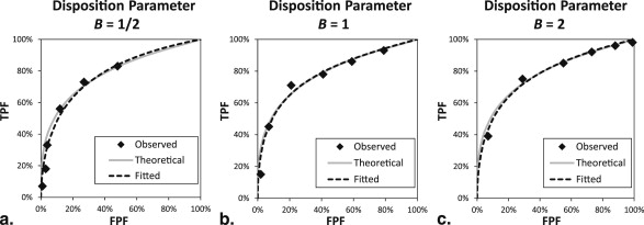
for c__i , n , which can be accomplished numerically to arbitrary precision. The exponent, B , is a positive categorization disposition parameter that controls where the thresholds appear on an ROC curve. We will consider the thresholds to be at baseline when B = 1. In this case, decision variables are equally spread among the categorical scores. Higher values of B lead to reduced categorization thresholds, which assigns more decision variables to higher scores. This moves the categorical operating points towards the upper right corner of the ROC curve. Conversely, lower values of B increase the categorization thresholds, which then move the observed operating points toward the lower left corner of the ROC curve. Effects of categorization disposition are shown in Figure A1 .

Get Radiology Tree app to read full this article<

Figures of Merit

Get Radiology Tree app to read full this article<

TPF=aFPF+(1−a)(1−Φ[cFPF−u]), TPF

FPF

(

−

)

(

−

[

FPF

−

]

)

where c FPF is the criterion associated with a given FPF value (ie,cFPF=Φ−1[1−FPF]) (

FPF

−

[

−FPF

]

) . The AUC is readily computed from the CBM parameters as

AUC=a2+(1−a)Φ(u2√). AUC

(

−

)

(

)

Get Radiology Tree app to read full this article<

FPFOOP=1−Φ[1uln(β−a1−a)−12u], FP

OOP

−

[

(

−

)

−

]

if β > a , and a < 1. The TPF at the optimal operating point, TPF OOP , is obtained by evaluating Equation A12 at FPF OOP . If β ≤ a , then the optimum point of the ROC curve is (FPF OOP , TPF OOP ) = (1,1). If a = 1 or u = 0 (in either case performance is at chance), then (FPF OOP , TPF OOP ) = (0,0) if β > 1, and (FPF OOP , TPF OOP ) = (1,1) if β < 1. The expected utility figure of merit, EU, is then

EU=TPFOOP−βFPFOOP. EU

OOP

−

OOP

Get Radiology Tree app to read full this article<

Power Analysis

Get Radiology Tree app to read full this article<

References

1. Gallas B.D., Chan H.P., D’Orsi C.J., et. al.: Evaluating imaging and computer-aided detection and diagnosis devices at the FDA. Acad Radiol 2012; 19: pp. 463-477.
2. Metz C.E.: Basic principles of ROC analysis. Semin Nucl Med 1978; 8: pp. 283-298.
3. Metz C.E.: ROC analysis in medical imaging: a tutorial review of the literature. Radiol Phys Technol 2008; 1: pp. 2-12.
4. Obuchowski N.A.: ROC analysis. AJR Am J Roentgenol 2005; 184: pp. 364-372.
5. Swets J.A., Pickett R.M.: Evaluation of diagnostic systems: methods from signal detection theory.1982.Academic PressNew York
6. Bamber D.: The area above the ordinal dominance graph and the area below the receiver operating characteristic graph. J Math Psychol 1975; 12: pp. 387-415.
7. Hanley J.A., McNeil B.J.: The meaning and use of the area under a receiver operating characteristic (ROC) curve. Radiology 1982; 143: pp. 29-36.
8. Metz C.E.: ROC methodology in radiologic imaging. Invest Radiol 1986; 21: pp. 720-733.
9. Hanley J.A.: Receiver operating characteristic (ROC) methodology: the state of the art. Crit Rev Diagnostic Imaging 1989; 29: pp. 307.
10. Green D.M., Swets J.A.: Signal detection theory and psychophysics.1966.WileyNew York
11. Peterson W., Birdsall T., Fox W.: The theory of signal detectability. IRE Professional Group on Information Theory 1954; 4: pp. 171-212.
12. Tanner W.P., Swets J.A.: A decision-making theory of visual detection. Psychol Rev 1954; 61: pp. 401-409.
13. Pauker S.G., Kassirer J.P.: Therapeutic decision making: a cost-benefit analysis. N Engl J Med 1975; 293: pp. 229-234.
14. Hilden J.: The area under the ROC curve and its competitors. Med Decis Making 1991; 11: pp. 95-101.
15. Moons K.G., Stijnen T., Michel B.C., et. al.: Application of treatment thresholds to diagnostic-test evaluation: an alternative to the comparison of areas under receiver operating characteristic curves. Med Decis Making 1997; 17: pp. 447-454.
16. Schisterman E.F., Perkins N.J., Liu A., et. al.: Optimal cut-point and its corresponding Youden Index to discriminate individuals using pooled blood samples. Epidemiology 2005; 16: pp. 73-81.
17. Schwartz W.B., Gorry G.A., Kassirer J.P., et. al.: Decision analysis and clinical judgment. Am J Med 1973; 55: pp. 459-472.
18. Lusted L.B.: Introduction to medical decision making.1968.C ThomasSpringfield, IL
19. Weinstein M.C., Fineberg H.V., Elstein A.S., et. al.: Clinical decision analysis.1980.SaundersPhiladelphia, PA
20. Sunshine J.: Contributed comment. Acad Radiol 1995; 2: pp. S72-S74.
21. Halpern E.J., Albert M., Krieger A.M., et. al.: Comparison of receiver operating characteristic curves on the basis of optimal operating points. Acad Radiol 1996; 3: pp. 245-253.
22. Wagner R.F., Beam C.A., Beiden S.V.: Reader variability in mammography and its implications for expected utility over the population of readers and cases. Med Decis Making 2004; 24: pp. 561-572.
23. Abbey C.K., Eckstein M.P., Boone J.M.: An equivalent relative utility metric for evaluating screening mammography. Med Decis Making 2010; 30: pp. 113-122.
24. Abbey CK, Eckstein MP, Boone JM. Estimating the relative utility of screening mammography. In Press: Medical Decision Making.
25. Roe C.A., Metz C.E.: Dorfman-Berbaum-Metz method for statistical analysis of multireader, multimodality receiver operating characteristic data: validation with computer simulation. Acad Radiol 1997; 4: pp. 298-303.
26. Dorfman D.D., Berbaum K.S., Metz C.E.: Receiver operating characteristic rating analysis. Generalization to the population of readers and patients with the jackknife method. Invest Radiol 1992; 27: pp. 723-731.
27. Roe C.A., Metz C.E.: Variance-component modeling in the analysis of receiver operating characteristic index estimates. Acad Radiol 1997; 4: pp. 587-600.
28. Beiden S.V., Wagner R.F., Campbell G., et. al.: Components-of-variance models for random-effects ROC analysis: the case of unequal variance structures across modalities. Acad Radiol 2001; 8: pp. 605-615.
29. Metz C.E., Kronman H.B.: Statistical significance tests for binormal ROC curves. J Math Psychol 1980; 22: pp. 218-243.
30. Swets J.A.: Form of empirical ROCs in discrimination and diagnostic tasks: implications for theory and measurement of performance. Psychol Bull 1986; 99: pp. 181-198.
31. Hillis S.L.: Simulation of unequal-variance binormal multireader ROC decision data: an extension of the Roe and Metz simulation model. Acad Radiol 2012; 19: pp. 1518-1528.
32. Hillis S.L., Berbaum K.S.: Using the mean-to-sigma ratio as a measure of the improperness of binormal ROC curves. Acad Radiol 2011; 18: pp. 143-154.
33. Dorfman D.D., Berbaum K.S.: A contaminated binormal model for ROC data: part III. Initial evaluation with detection ROC data. Acad Radiol 2000; 7: pp. 438-447.
34. Dorfman D.D., Berbaum K.S.: A contaminated binormal model for ROC data: Part II. A formal model. Acad Radiol 2000; 7: pp. 427-437.
35. Dorfman D.D., Berbaum K.S., Brandser E.A.: A contaminated binormal model for ROC data: part I. Some interesting examples of binormal degeneracy. Acad Radiol 2000; 7: pp. 420-426.
36. Hillis S.L., Berbaum K.S., Metz C.E.: Recent developments in the Dorfman-Berbaum-Metz procedure for multireader ROC study analysis. Acad Radiol 2008; 15: pp. 647-661.

Statistical Power Considerations for a Utility Endpoint in Observer Performance Studie s

Rationale and Objectives

Materials and Methods

Results

Conclusion

Materials and methods

A Roe and Metz Type Simulation

AUC and Utility Endpoints

Scope of Studies

Results

Discussion

Appendix

Simulation Model and Components of Variance

Unequal Variance Model

Generating Discrete Ratings

Figures of Merit

Power Analysis

References

Further Reading

A Brief History of Free-Response Receiver Operating Characteristic Paradigm Data Analysis

An Additive Selection of Markers to Improve Diagnostic Accuracy Based on a Discriminatory Measure

An Examination of Data Confidentiality and Disclosure Issues Related to Publication of Empirical ROC Curves