Teaching Radiology Physics Interactively with Scientific Notebook Software

Rationale and Objectives

The goal of this study is to demonstrate how the teaching of radiology physics can be enhanced with the use of interactive scientific notebook software.

Methods

We used the scientific notebook software known as Project Jupyter, which is free, open-source, and available for the Macintosh, Windows, and Linux operating systems.

Results

We have created a scientific notebook that demonstrates multiple interactive teaching modules we have written for our residents using the Jupyter notebook system.

Conclusions

Scientific notebook software allows educators to create teaching modules in a form that combines text, graphics, images, data, interactive calculations, and image analysis within a single document. These notebooks can be used to build interactive teaching modules, which can help explain complex topics in imaging physics to residents.

Introduction

The American Board of Radiology (ABR) Core Examination assesses knowledge of physics as part of its overall testing in clinical radiology. Physics questions are integrated into each category of this examination . Topics emphasized include image quality, artifacts, radiation dose, and patient safety for each modality or subspecialty organ system. Radiology residencies therefore include instruction in physics as part of the residency curriculum. However, imparting an adequate understanding of imaging physics remains a challenging task.

Zhang et al. showed that a hands-on exposure to clinically oriented physics was not only well received by radiology residents but also improved their understanding of the material. It occurred to us that such physical hands-on experiences could be supplemented or possibly even replaced by suitable simulations.

Get Radiology Tree app to read full this article<

Methods

Get Radiology Tree app to read full this article<

Using Jupyter

Get Radiology Tree app to read full this article<

Results

Get Radiology Tree app to read full this article<

Nuclear Medicine

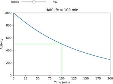
Module 1. Simple Radioactive Decay

Get Radiology Tree app to read full this article<

A(t)=A0e−λt, A

(

)

−

where A 0 is the initial activity, t is time, and λ is the decay constant—the probability that a radioatom will decay per unit time . This decay constant is related to the isotope’s half-life (t12) (

) —the time when 50% of the radioatoms present will have decayed—as shown in Equation 2 :

t12=ln(2)λ. t

(

)

Half-life has direct implications in nuclear medicine imaging, radiation therapy, and radiation safety. For example, the half-life can make it relatively simple to calculate how much of a radioisotope will be left after a given time. For example, technetium-99m ( 99m Tc) has a half-life of about 6 hours. Therefore, after 24 hours, the remaining amount of 99m Tc will be 1/2 × 1/2 × 1/2 × 1/2 or 1/16 of the original amount.

Get Radiology Tree app to read full this article<

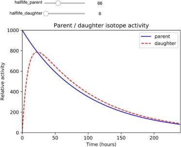
Module 2. Technetium Generator Simulation

Get Radiology Tree app to read full this article<

99Mo→λA99mTc→λB99Tc 99

→

Get Radiology Tree app to read full this article<

parent→λAdaughter→λBgranddaughter parent

→

daughter

→

granddaughter

can be expressed by the Bateman equation (Eq. 5 ) :

Aparent=λdaughterλdaughter−λparentAparent(0)(e−λparentt−e−λdaughtert). A

parent

daughter

−

parent

(

)

(

−

parent

−

daughter

)

Get Radiology Tree app to read full this article<

Secular equilibrium

Get Radiology Tree app to read full this article<

Transient equilibrium

Get Radiology Tree app to read full this article<

Ultrasound

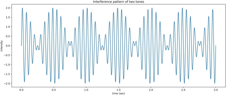
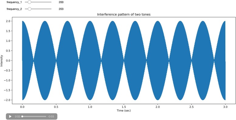
Module 3. Sound Interference Patterns

Get Radiology Tree app to read full this article<

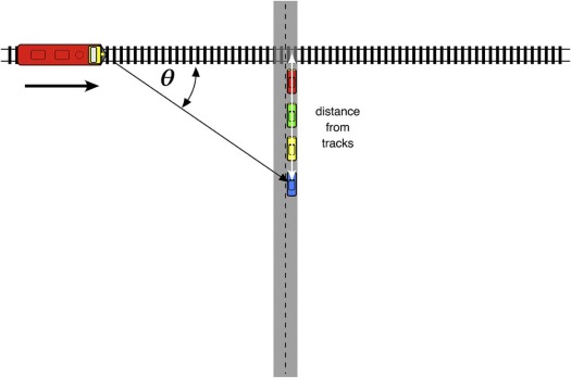
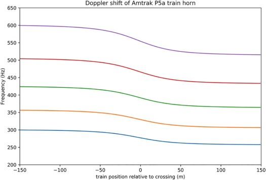
Module 4. Doppler Shift Simulation

Get Radiology Tree app to read full this article<

fobs=forig×cc+Vsource, f

orig

source

where f orig is the original frequency, f obs is the observed frequency, c is the velocity of sound in a medium, and V source is the speed of the source.

Get Radiology Tree app to read full this article<

Vradial=Vsource×cosθ, V

radial

source

cos

where θ is the angle between the source’s forward direction of travel and the line of sight from the source to the observer.

Get Radiology Tree app to read full this article<

Magnetic Resonance Imaging

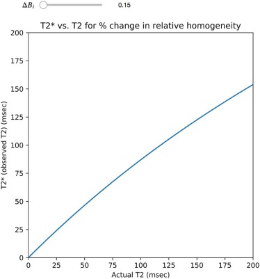
Module 5: T2 vs T2*

Get Radiology Tree app to read full this article<

Mxy(t)=M0e−tT2 M

(

)

−

Get Radiology Tree app to read full this article<

1T2*=1T2+1T2i. 1

Get Radiology Tree app to read full this article<

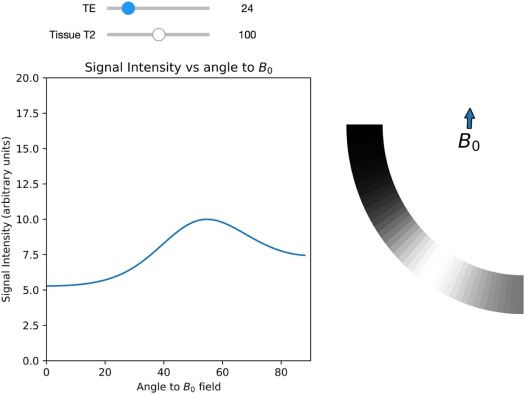
Module 6: Magic Angle Effect in a Tendon

Get Radiology Tree app to read full this article<

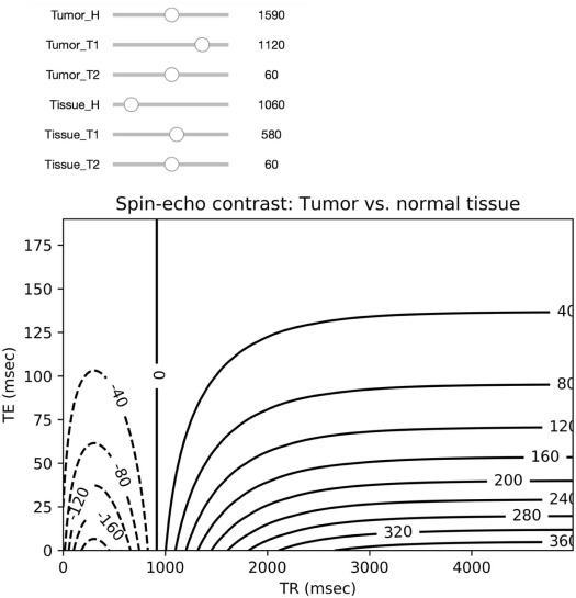
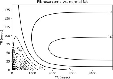
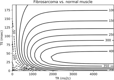
Module 7: MR Contrast Optimization

Get Radiology Tree app to read full this article<

Intensity=H⋅e−TET2(1−2e−(TR−3τ)T1+2e−(TR−τ)T1−e−TRT1), Intensity

⋅

−

(

−

(

−

)

−

(

−

)

−

)

where H is the local hydrogen density, T1 is the longitudinal magnetic relaxation constant, T2 is the transverse magnetic relaxation constant, TR is the pulse repetition time, TE is the echo delay, and τ is the time between the first 90° radiofrequency pulse and the first 180° radiofrequency pulse in the spin-echo pulse train.

Get Radiology Tree app to read full this article<

contrast=Intensitytumor−Intensitybackground contrast

Intensit

tumor

−

Intensit

background

Get Radiology Tree app to read full this article<

TABLE 1

Measured Values of Tissue Parameters From the Literature

Tissue H T1 (ms) T2 (ms) Normal fat 1170–1580 214–242 46–58 Normal marrow 1280–1410 210–246 51–60 Normal muscle 1000 456–520 28–40 Fibrosarcoma 1180 991 71 Giant cell tumor 950 965 68 Osteogenic sarcoma 1360–1990 991–1213 58–62

Get Radiology Tree app to read full this article<

Discussion

Get Radiology Tree app to read full this article<

Conclusions

Get Radiology Tree app to read full this article<

References

1. American Board of Radiology : Core exam. Available at https://www.theabr.org/diagnostic-radiology/initial-certification/core-exam#exam-categories
2. Zhang J., Hardy P.A., DiSantis D.J., et. al.: Hands-on physics education of residents in diagnostic radiology. Acad Radiol 2017; 24: pp. 677-681.
3. Shen H.: Interactive notebooks: sharing the code. Nature 2014; 515: pp. 151-152.
4. Van Noorden R.: My digital toolbox: Ecologist Ethan White on interactive notebooks. Nature 2014; Available at http://www.nature.com/news/my-digital-toolbox-ecologist-ethan-white-on-interactive-notebooks-1.16015
5. Osipov D.: The rise of data science notebooks. Available at https://www.datanami.com/2016/05/04/rise-data-science-notebooks/
6. Wolfram Language and System Documentation Center : Using a notebook interface. Available at https://reference.wolfram.com/language/tutorial/UsingANotebookInterface.html
7. Maplesoft : Maplesoft - Software for Mathematics, Online Learning, Engineering. Available at http://www.maplesoft.com
8. Matlab : MathWorks - Makers of MATLAB and Simulink. Available at https://www.mathworks.com
9. Project Jupyter : Project Jupyter Home. Available at http://jupyter.org
10. RStudio Team : Integrated development environment for R.2015.RStudio, Inc.Boston, MA Available at http://www.rstudio.com/
11. Pérez F., Granger B.E.: IPython: a system for interactive scientific computing. Comput Sci Eng 2007; 9: pp. 21-29. Available at http://ipython.org
12. Richardson M.L., Amini B.: Scientific notebook software: applications for radiology. Curr Probl Diagn Radiol 2017; epub ahead of print
13. van der Walt S., Schönberger J.L., Nunez-Iglesias J., et. al.: Scikit-image: image processing in Python. Peer J 2014; 2: pp. e453. https://doi.org/10.7717/peerj.453
14. van der Walt S., Colbert S.C., Varoquaux G.: The NumPy array: a structure for efficient numerical computation. Comput Sci Eng 2011; 13: pp. 22-30.
15. Gruber J.: Markdown: Syntax. Available at https://daringfireball.net/projects/markdown/syntax
16. GitHub contributors : Writing on GitHub/Basic writing and formatting syntax. Available at https://help.github.com/articles/basic-writing-and-formatting-syntax/
17. Mittelbach F., Goossens M.: The LaTeX companion.2nd ed.2004.Addison-WesleyBoston, MA
18. Groch M.W.: Radioactive decay. Radiographics 1998; 18: pp. 1247-1256.
19. Wikipedia : Doppler effect—Wikipedia, the free encyclopedia. Available at https://en.wikipedia.org/w/index.php?title=Doppler_effect&oldid=831208270
20. Chappell K.E., Robson M.D., Stonebridge-Foster A., et. al.: Magic angle effects in MR neurography. AJNR Am J Neuroradiol 2004; 25: pp. 431-440.
21. Pérez F., Granger B.E., Hunter J.D.: Python: an ecosystem for scientific computing. Comput Sci Eng 2011; 13: pp. 13-21.
22. Erickson S.J., Cox I.H., Hyde J.S., et. al.: Effect of tendon orientation on MR imaging signal intensity: a manifestation of the “magic angle” phenomenon. Radiology 1991; 181: pp. 389-392.
23. Hayes C.W., Parellada J.A.: The magic angle effect in musculoskeletal MR imaging. Top Magn Reson Imaging 1996; 8: pp. 51-56.
24. Marshall H., Howarth C., Larkman D.J., et. al.: Contrast-enhanced magic-angle MR imaging of the Achilles tendon. AJR Am J Roentgenol 2002; 179: pp. 187-192.
25. Oatridge A., Herlihy A., Thomas R.W., et. al.: Magic angle imaging of the Achilles tendon in patients with chronic tendinopathy. Clin Radiol 2003; 58: pp. 384-388.
26. Richardson M.L., Amparo E.G., Gillespy T., et. al.: Theoretical considerations for optimizing intensity differences between primary musculoskeletal tumors and normal tissue with spin-echo magnetic resonance imaging. Invest Radiol 1985; 20: pp. 492-497.
27. Mitchell M.R., Conturo T.E., Gruber T.J., et. al.: AUR memorial award. Two computer models for selection of optimal magnetic resonance imaging (MRI) pulse sequence timing. Invest Radiol 1984; 19: pp. 350-360.
28. AAPM Subcommittee of Physics Education of Physics : Diagnostic radiology physics curriculum. Available at http://www.aapm.org/education/documents/Curriculum.pdf
29. Jacobs C.T., Gorman G.J., Rees H.E., et. al.: Experiences with efficient methodologies for teaching computer programming to geoscientists. J Geosci Educ 2016; 64: pp. 183-198.
30. Milas J.: Jupyter in the classroom. Available at https://deephorizons.github.io/2016/06/06/jupyter-in-the-classroom/
31. Jones B., Beazley D.: Python cookbook—recipes for mastering Python 3.3rd ed.2013.O’ReillySebastopol, CA Available at http://shop.oreilly.com/product/0636920027072.do
32. Chang W.: Cookbook for R.. Available at http://www.cookbook-r.com
33. Teetor P.: R cookbook. O’Reilly. Available at http://shop.oreilly.com/product/9780596809164.do
34. Stack Overflow Contributors : Stack overflow. Available at https://stackoverflow.com

Teaching Radiology Physics Interactively with Scientific Notebook Software

Rationale and Objectives

Methods

Results

Conclusions

Introduction

Methods

Using Jupyter

Results

Nuclear Medicine

Module 1. Simple Radioactive Decay

Module 2. Technetium Generator Simulation

Secular equilibrium

Transient equilibrium

Ultrasound

Module 3. Sound Interference Patterns

Module 4. Doppler Shift Simulation

Magnetic Resonance Imaging

Module 5: T2 vs T2*

Module 6: Magic Angle Effect in a Tendon

Module 7: MR Contrast Optimization

Discussion

Conclusions

References

Further Reading

(Lack of) Measurable Clinical or Knowledge Gains From Resident Participation in Noon Conference

Attitudes of Radiology Program Directors Toward MD-PhD Trainees, Resident Research Productivity, and Dedicated Research Time

Best Practices From the APDR