
Rationale and Objectives
We showed previously that maximum-likelihood (ML) and Bayesian (with a flat prior on a common parameterization of the model) estimates of “proper” binormal receiver operating characteristic (ROC) curves produce similar results. We propose a new prior that is flat over the area under the ROC curve (AUC) and investigate its effect on the Bayesian estimates.
Materials and Methods
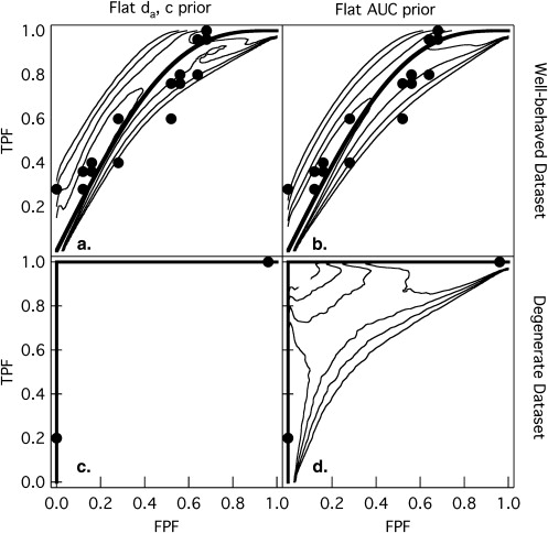
In two simulation studies, we compared Bayesian estimation of the AUC with the two prior probability distributions against ML estimation in terms of root mean squared error (RMSE) and the coverage of 95% confidence (or credible) intervals (both abbreviated CIs). In the first study, we simulated categorical data that tend to be “well-behaved” and produce ROC curve estimates that most would consider reasonable. In the second study, we simulated coarsely discretized categorical data that often included so-called degenerate datasets that cause the ML estimate to be the perfect ROC curve.
Results
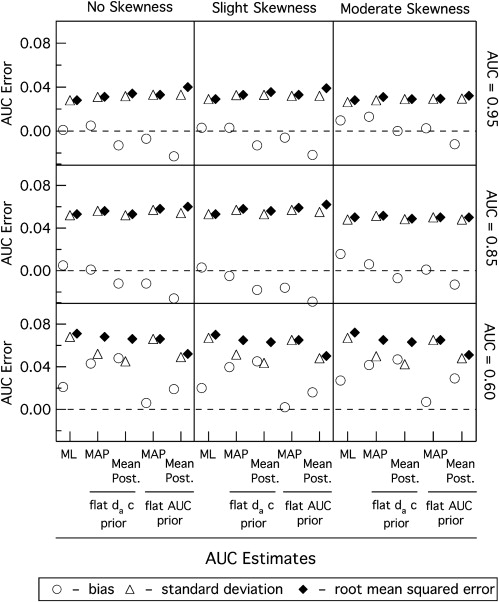
For the well-behaved datasets, all three AUC estimates were similar in terms of RMSE and 95% CI coverage. For the coarsely discretized datasets, the RMSE of ML was consistently greater than that of Bayesian estimation and the 95% CI coverage of ML estimation was consistently below nominal, whereas the 95% CI coverage of Bayesian estimation was consistently equal to, or greater than, nominal.
Conclusion
Bayesian estimation with a flat prior on the AUC can provide reasonable inference from datasets with coarsely categorized data that are prone to be degenerate and produce results similar to other estimation methods on well-behaved datasets.
Receiver operating characteristic (ROC) analysis is a fundamental method for the evaluation of diagnostic accuracy . An ROC curve is a plot of true-positive fraction (TPF, or sensitivity) versus false-positive fraction (FPF, or 1-specificity). The conventional binormal model for ROC analysis provides satisfactory ROC curve fits in a wide variety of practical situations . However, except for ROC curves that are symmetrical with respect to the negative 45° line in the ROC plot, the conventional binormal model produces ROC curve estimates that contain “hooks” (ie, a change in the ROC curve curvature [eg, from convex to concave], which for the conventional binormal model implies that a portion of the ROC curve falls below the “guessing line” defined by TPF = FPF). These ROC curve estimates are considered unsatisfactory because hooks indicate diagnostic accuracies that are worse than guessing . ROC models that describe ROC curves guaranteed to have a monotonically decreasing slope are known as “proper” ROC models . In this article, we focus on the so-called “proper” binormal model .
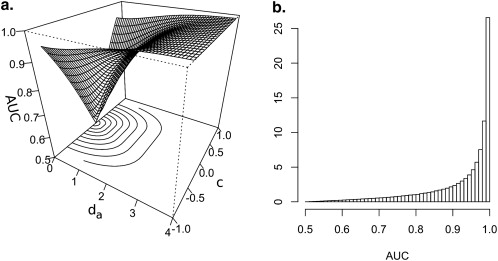
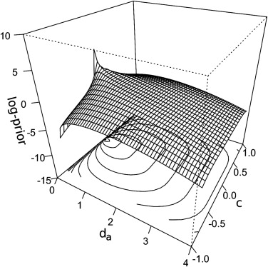
Previously (Zur RM, unpublished data, 2010), we compared maximum-likelihood (ML) and Bayesian estimates of “proper” binormal ROC curves. The Bayesian estimates were based on a prior probability distribution that is flat (ie, constant) over the most common parameterization of the proper binormal model . Prior probability distributions are a well-known characteristic of Bayesian estimation and they incorporate information obtained independently from the data at hand . Because of that, priors are expected either to improve estimations or to bias them. We showed (Zur RM, unpublished data, 2010) that the Bayesian and ML estimates are similar in terms of root mean squared error (RMSE) for the area under the ROC curve (AUC), TPF values at fixed FPF values and FPF values at fixed TPF values. In this article, we evaluate the effect on Bayesian estimation of proper binormal ROC curves of a new prior that is not flat over the most common parameterization of the proper binormal model but, rather, flat over the AUC values. We refer to both of these flat priors as low information because they do contain information (as will be demonstrated later through reparameterization) and can affect ROC analysis. Our motivation was that, whereas a prior flat on the curve parameters is expected to influence minimally the estimation of the curve parameters, it is probably more desirable to influence minimally the estimation of the AUC—the most commonly reported ROC summary index in radiological research . It is not possible to impose a prior that is simultaneously flat on both the curve parameters and the AUC because the curve parameters and the AUC are nonlinear functions of each other . Therefore, a tradeoff is unavoidable. Although the effect of prior information or preconceived views is usually not discussed in the context of ROC curve estimation, a review of the radiological literature that reports ROC analysis shows that prior experience and belief do seem to influence our understanding and acceptance of ROC curve estimates .
Background
The “Proper” Binormal ROC Model
Get Radiology Tree app to read full this article<
Get Radiology Tree app to read full this article<
ML Estimation of the “Proper” Binormal ROC Model
Get Radiology Tree app to read full this article<
## Bayesian Estimation of the “Proper” Binormal ROC Model
Get Radiology Tree app to read full this article<
p(da,c,{vci}|D)=L(da,c,{vci};D)p(da,c,{vci})p(D), p
(
d
a
,
c
,
{
v
c
i
}
|
D
)
=
L
(
d
a
,
c
,
{
v
c
i
}
;
D
)
p
(
d
a
,
c
,
{
v
c
i
}
)
p
(
D
)
,
where p ( d a , c , { v ci }) is the prior probability distribution and p ( **D ) is the marginal likelihood . The marginal likelihood can be considered as a normalization constant, which does not affect most estimates of the posterior probability distribution . Therefore, Bayesian estimation focuses on the probability of the model given the data (ie, the posterior probability distribution), rather than on the probability of the data given a model (ie, the likelihood function). However, as shown in equation , a prior probability distribution is required to estimate the posterior probability distribution. It is not always clear what the best or even a reasonable prior probability distribution is. Furthermore, we are often interested in indices that are different from, or in addition to, the parameters that we estimate directly. In such instances, even after necessary transformations , we sometimes find that a prior probability distribution that is reasonable for one set of parameters does not appear to be reasonable for other parameters of interest. Moreover, to estimate a high-dimensional, nonstandard, probability distribution, as is often required with Bayesian estimation, can be computationally challenging. Here, we use Markov chain Monte Carlo (MCMC) algorithms for that purpose .**
Get Radiology Tree app to read full this article<
## MCMC Estimation of the Bayesian Posterior Probability Distribution
Get Radiology Tree app to read full this article<
Get Radiology Tree app to read full this article<
## Degenerate Datasets Compatible with the Perfect ROC Curve
Get Radiology Tree app to read full this article<
Get Radiology Tree app to read full this article<## Materials and methods
## The Prior Probability Distributions
Get Radiology Tree app to read full this article<
Get Radiology Tree app to read full this article<
Get Radiology Tree app to read full this article<
Get Radiology Tree app to read full this article<
Get Radiology Tree app to read full this article<
## Simulation Studies
Get Radiology Tree app to read full this article<
Get Radiology Tree app to read full this article<
Get Radiology Tree app to read full this article<
Get Radiology Tree app to read full this article<
## Analysis of Simulation Study Datasets
Get Radiology Tree app to read full this article<
## Results
Get Radiology Tree app to read full this article<
Get Radiology Tree app to read full this article<
Get Radiology Tree app to read full this article<
Get Radiology Tree app to read full this article<
Get Radiology Tree app to read full this article<
Get Radiology Tree app to read full this article<
Get Radiology Tree app to read full this article<
Get Radiology Tree app to read full this article<
Get Radiology Tree app to read full this article<
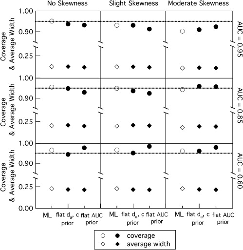
![Figure 7, Comparison of maximum-likelihood (ML) and Bayesian (with the flat prior on the area under the curve [AUC]) estimations in term of the coverage and width of the 95% CIs of the AUC estimates from coarsely categorized datasets that are prone to be degenerate, simulated from three population receiver operating characteristic curves and with three different probabilities of producing degenerate datasets. Uncertainties in the estimates of the coverage are approximately the size of the data points. Bars on the average width represent the range containing 95% of the individual values of the width.](https://storage.googleapis.com/dl.dentistrykey.com/clinical/TheEffectofTwoPriorsonBayesianEstimationofProperBinormalROCCurvesfromCommonandDegenerateDatasets/6_1s20S1076633210001765.jpg)
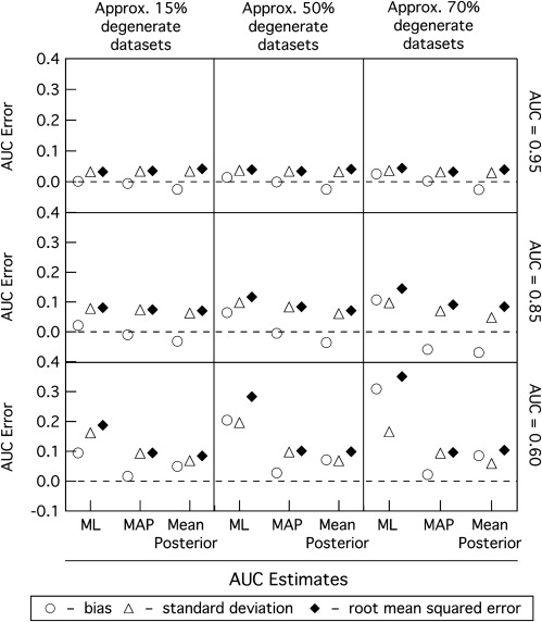
![Figure 8, Comparison between maximum-likelihood (ML) and Bayesian mean-posterior (with the flat prior on the area under the curve [AUC]) estimates of the AUC ( solid lines ) and its 95% CIs ( points ) on coarsely categorized datasets that are prone to be degenerate simulated from three population receiver operating characteristic (ROC) curves (probability of producing degenerate dataset approximately 50%). The AUC estimates are sorted in increasing order. The dashed lines indicate the AUC values of the population ROC curves.](https://storage.googleapis.com/dl.dentistrykey.com/clinical/TheEffectofTwoPriorsonBayesianEstimationofProperBinormalROCCurvesfromCommonandDegenerateDatasets/7_1s20S1076633210001765.jpg)
Get Radiology Tree app to read full this article<
## Discussion
Get Radiology Tree app to read full this article<
Get Radiology Tree app to read full this article<
Get Radiology Tree app to read full this article<
Get Radiology Tree app to read full this article<
Get Radiology Tree app to read full this article<
Get Radiology Tree app to read full this article<
Get Radiology Tree app to read full this article<
Get Radiology Tree app to read full this article<
Get Radiology Tree app to read full this article<
Get Radiology Tree app to read full this article<
## Acknowledgments
Get Radiology Tree app to read full this article<
## Appendix
Get Radiology Tree app to read full this article<
p(AUC)=2. p
(
A
U
C
)
=
2
.
Get Radiology Tree app to read full this article<
Get Radiology Tree app to read full this article<
p(c|AUC)=12tan(2π(AUC−0.5)), p
(
c
|
A
U
C
)
=
1
2
tan
(
2
π
(
A
U
C
−
0.5
)
)
,
and the joint probability is
p(AUC,c)=p(c|AUC)p(AUC)=1tan(2π(AUC−0.5)). p
(
A
U
C
,
c
)
=
p
(
c
|
A
U
C
)
p
(
A
U
C
)
=
1
tan
(
2
π
(
A
U
C
−
0.5
)
)
.
Get Radiology Tree app to read full this article<
Get Radiology Tree app to read full this article<
J(da,c)=∣∣∣∣∂AUC∂da∂c∂da∂AUC∂c∂c∂c∣∣∣∣=∂AUC∂da∂c∂c−∂AUC∂c∂c∂da=∂AUC∂da=12π√e−d2a4⎡⎣⎢1−2Θ⎛⎝⎜c2−1c2+1da2−2(c2−1c2+1)2√⎞⎠⎟⎤⎦⎥, J
(
d
a
,
c
)
=
|
∂
A
U
C
∂
d
a
∂
A
U
C
∂
c
∂
c
∂
d
a
∂
c
∂
c
|
=
∂
A
U
C
∂
d
a
∂
c
∂
c
−
∂
A
U
C
∂
c
∂
c
∂
d
a
=
∂
A
U
C
∂
d
a
=
1
2
π
e
−
d
a
2
4
[
1
−
2
Θ
(
c
2
−
1
c
2
+
1
d
a
2
−
2
(
c
2
−
1
c
2
+
1
)
2
)
]
,
where Θ is the cumulative standard normal function. Therefore, the prior probability distribution over d a and c that corresponds to a prior probability distribution that is marginally flat over the AUC is
p(da,c)=p(AUC,c)∂(AUC,c)∂(da,c)=1tan(2π(AUC−0.5))12π√e−d2a4⎡⎣⎢1−2Θ⎛⎝⎜c2−1c2+1da2−2(c2−1c2+1)2√⎞⎠⎟⎤⎦⎥. p
(
d
a
,
c
)
=
p
(
A
U
C
,
c
)
∂
(
A
U
C
,
c
)
∂
(
d
a
,
c
)
=
1
tan
(
2
π
(
A
U
C
−
0.5
)
)
1
2
π
e
−
d
a
2
4
[
1
−
2
Θ
(
c
2
−
1
c
2
+
1
d
a
2
−
2
(
c
2
−
1
c
2
+
1
)
2
)
]
.
Get Radiology Tree app to read full this article<
Get Radiology Tree app to read full this article<
## References
- 1. Pepe M.S.: The statistical evaluation of medical tests for classification and prediction.2003.Oxford University PressNew York, NY
- 2. Zhou X.-H., Obuchowski N.A., McClish D.K.: Statistical methods in diagnostic medicine.2002.Wiley-InterscienceNew York, NY
- 3. Wagner R.F., Metz C.E., Campbell G.: Assessment of medical imaging systems and computer aids: a tutorial review. Acad Radiol 2007; 14: pp. 723-748.
- 4. Hanley J.A.: The robustness of the “binormal” assumptions used in fitting ROC curves. Med Decis Making 1988; 8: pp. 197-203.
- 5. Hanley J.A.: Receiver operating characteristic (ROC) methodology: the state of the art. Crit Rev Diagn Imaging 1989; 29: pp. 307-335.
- 6. Swets J.A.: Indices of discrimination or diagnostic accuracy: their ROCs and implied models. Psychol Bull 1986; 99: pp. 100-117.
- 7. Swets J.A., Pickett R.M.: Evaluation of diagnostic systems: methods from signal detection theory.1982.Academic PressNew York, NY
- 8. Lloyd C.J.: Estimation of a convex ROC curve. Stat Probabil Lett 2002; 59: pp. 99-111.
- 9. Green D.M., Swets J.A.: Signal detection theory and psychophysics.1966.WileyNew York, NY
- 10. Metz C.E.: Some practical issues of experimental-design and data-analysis in radiological ROC studies. Invest Radiol 1989; 24: pp. 234-245.
- 11. Metz C.E., Pan X.: “Proper” binormal ROC curves: theory and maximum-likelihood estimation. J Math Psychol 1999; 43: pp. 1-33.
- 12. Pesce L.L., Metz C.E.: Reliable and computationally efficient maximum-likelihood estimation of “proper” binormal ROC curves. Acad Radiol 2007; 14: pp. 814-829.
- 13. Gelman A.: Bayesian data analysis.2nd ed.2004.Chapman & Hall/CRCBoca Raton, FL
- 14. Woodworth G.G.: Biostatistics: a Bayesian introduction.2005.Wiley-InterscienceHoboken, NJ
- 15. Shiraishi J., Pesce L.L., Metz C.E., Doi K.: Experimental design and data analysis in receiver operating characteristic studies: lessons learned from papers published in Radiology from 1997 to 2006. Radiology 2009; 253: pp. 822-830.
- 16. Papoulis A., Pillai S.U.: Probability, random variables, and stochastic processes.4th ed.2002.McGraw-HillBoston, Ma
- 17. Metz C.E.: Basic principles of ROC analysis. Semin Nucl Med 1978; 8: pp. 283-298.
- 18. Ogilvie J.C., Creelman C.D.: Maximum-likelihood estimation of receiver operating characteristic curve parameters. J Math Psychol 1968; 5: pp. 377-391.
- 19. Dorfman D.D., Alf E.: Maximum-likelihood estimation of parameters of signal-detection theory and determination of confidence intervals-rating-method data. J Math Psychol 1969; 6: pp. 487-496.
- 20. Metz C.E., Herman B.A., Shen J.H.: Maximum likelihood estimation of receiver operating characteristic (ROC) curves from continuously-distributed data. Stat Med 1998; 17: pp. 1033-1053.
- 21. Kendall M.G., Stuart A., Ord J.K., Arnold S.F., O’Hagan A.: Kendall’s advanced theory of statistics: classical inference and the linear model.6th ed.1994.Hodder ArnoldNew York, NY
- 22. Liu J.S.: Monte Carlo strategies in scientific computing.2001.SpringerNew York, NY
- 23. Robert C.P., Casella G.: Monte Carlo statistical methods.2nd ed.2004.SpringerNew York, NY
- 24. Chib S., Greenberg E.: Understanding the Metropolis-Hastings algorithm. Am Stat 1995; 49: pp. 327-335.
- 25. Neal R.M.: Slice sampling. Ann Stat 2003; 31: pp. 705-741.
- 26. Bamber D.: The area above the ordinal dominance graph and the area below the receiver operating characteristic graph. J Math Psychol 1975; 12: pp. 387-415.
- 27. Scott D.W.: Multivariate density estimation: theory, practice, and visualization.1992.WileyNew York, NY
- 28. Little R.J.A., Rubin D.B.: Statistical analysis with missing data.2nd ed.2002.WileyHoboken, NJ
- 29. Obuchowski N.A., Lieber M.L.: Confidence bounds when the estimated ROC area is 1.0. Acad Radiol 2002; 9: pp. 526-530.
- 30. Wagner R.F., Beiden S.V., Metz C.E.: Continuous versus categorical data for ROC analysis: some quantitative considerations. Acad Radiol 2001; 8: pp. 328-334.