
Rationale and Objectives
Traditionally, maximum gallbladder wall thickness is measured at a single point on ultrasonography. The purpose of this work was to develop an automated technique to measure the thickness of the gallbladder wall over the entire gallbladder surface using computer tomography (CT).
Materials and Methods
Subjects who had (5-mm) thick and thin (2.5-mm) reconstruction through the abdomen were selected from a research database. Their volumetric computed tomographic images were acquired using a multidetector GE Medical Systems LightSpeed 16 scanner at 120 kVp, ≈250 mAs, with standard filter reconstruction algorithm and segmented in three dimensions. Two segmentation boundaries were obtained, an inner and an outer boundary of the gallbladder wall. The thickness of the wall was quantified by computing the distance between the boundaries over the entire volume using Laplace’s equation from mathematical physics. The distance between the surfaces is found by computing normalized gradients that form a vector field, representing tangent vectors along field lines connecting both boundaries. The Laplacian technique was compared with the well-known Euclidean distance transformation (EDT) technique that provides a three-dimensional Euclidean distance mapping between the two extracted surfaces.
Results
The technique was tested on 10 subjects who had thin- and thick-section computed tomographic datasets reconstructed from a single scan. The mean thickness for the thick- and thin-section CT using Laplace was 3.18 and 2.93 mm, respectively. The smooth transition between surfaces resulting from the Laplace technique resulted in a coefficient of variation that was less than 1% compared to EDT.
Conclusions
EDT technique is very sensitive to imperfect segmentations, resulting in higher variation compared to the Laplacian technique. The smooth transition between surfaces makes the Laplacian technique more robust compared to EDT for the measurement of CT gallbladder thickness.
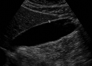
Thickening of the gallbladder wall is a relatively frequent finding in diagnostic imaging studies. Historically, a thick-walled gallbladder has been regarded as evidence of primary gallbladder disease, and it is a well-known feature of many gallbladder-related diseases. The gallbladder wall is usually perceptible as a thin attenuating rim of soft tissue as shown in Figure 1 . Although its thickness depends upon the degree of gallbladder distention, 3 mm is regarded as the upper limit of normal thickening ( ).
 Open full size image
Figure 1
Gallbladder wall shown by arrow.
Get Radiology Tree app to read full this article<
Get Radiology Tree app to read full this article<
Get Radiology Tree app to read full this article<
 Open full size image
Figure 2
Example of a computed tomographic scan with superimposed segmentation of the gallbladder wall. Although the wall thickness indicated at points A and B appears nearly the same, subsequent analysis reveals that A is thicker than B due to the three-dimensional nature of the gallbladder. It is also worth noting that even though two patients can have a similar maximum diameter, the overall wall thickness may be clearly different.
Get Radiology Tree app to read full this article<
Methods
Tissue Segmentation and Preparation of Boundaries
Get Radiology Tree app to read full this article<
CT Wall Thickness Calculation
Get Radiology Tree app to read full this article<
Get Radiology Tree app to read full this article<
Get Radiology Tree app to read full this article<
Get Radiology Tree app to read full this article<
∇2Ψ=∂2Ψ∂2x2+∂2Ψ∂2y2+∂2Ψ∂2z2. ∇
2
Ψ
=
∂
2
Ψ
∂
2
x
2
+
∂
2
Ψ
∂
2
y
2
+
∂
2
Ψ
∂
2
z
2
.
Get Radiology Tree app to read full this article<
Get Radiology Tree app to read full this article<
Ψi+1(x,y,z)=[Ψi(x+Δx,y,z)+Ψi(x−Δx,y,z)+Ψi(x,y+Δy,z)+Ψi(x,y−Δy,z)+Ψi(x,y,z+Δz)+Ψi(x,y,z−Δz)]/6 Ψ
i
+
1
(
x
,
y
,
z
)
=
[
Ψ
i
(
x
+
Δ
x
,
y
,
z
)
+
Ψ
i
(
x
−
Δ
x
,
y
,
z
)
+
Ψ
i
(
x
,
y
+
Δ
y
,
z
)
+
Ψ
i
(
x
,
y
−
Δ
y
,
z
)
+
Ψ
i
(
x
,
y
,
z
+
Δ
z
)
+
Ψ
i
(
x
,
y
,
z
−
Δ
z
)
]
/
6
where Ψi Ψ
i is the value at x,y,z x
,
y
,
z when Laplace is solved during the i th iteration. Convergence is measured by the total field energy over all voxels given by:
εi=∑[(ΔΨi/Δx)2+(ΔΨi/Δy)2+(ΔΨi/Δz)2]12. ε
i
=
∑
[
(
Δ
Ψ
i
/
Δ
x
)
2
+
(
Δ
Ψ
i
/
Δ
y
)
2
+
(
Δ
Ψ
i
/
Δ
z
)
2
]
1
2
.
Get Radiology Tree app to read full this article<
Get Radiology Tree app to read full this article<
E=−∇Ψ Ε
=
−
∇
Ψ
that is normalized to
N=E/∥E∥ Ν
=
Ε
/
∥
Ε
∥
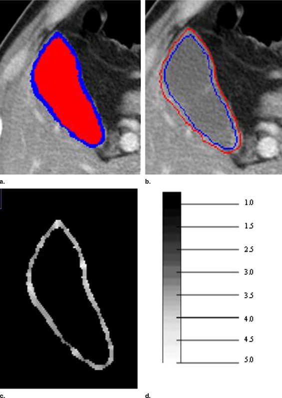
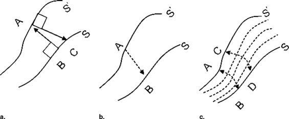
where N represents a unit vector field defined everywhere between S and S′ that always points perpendicular to the sublayer on which it sits. After computing N, “field lines” or “streamlines” are computed by starting at any point on S and integrating N using finite differences, derived from Taylor series expansions ( ). The resulting thickness map is shown in Figure 4 c alongside a scale.
Get Radiology Tree app to read full this article<
Experimental Testing
Data acquisition
Get Radiology Tree app to read full this article<
Get Radiology Tree app to read full this article<
Analysis
Get Radiology Tree app to read full this article<
cv=σμ. c
v
=
σ
μ
.
Get Radiology Tree app to read full this article<
Results
Get Radiology Tree app to read full this article<
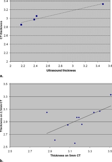
Table 1
Coefficient of Variation in Percentage for Different Methods of Thickness Measurement
EDT1 EDT2 Laplace Thick section CT 4.05 3.78 2.54 Thin section CT 3.55 3.11 2.09
CT, computed tomography; EDT, Euclidean distance transformation.
Get Radiology Tree app to read full this article<
Discussion
Get Radiology Tree app to read full this article<
Get Radiology Tree app to read full this article<
Conclusion
Get Radiology Tree app to read full this article<
References
1. Zissin R., Osadchy A., Shapiro M., Gayer G.: CT of a thickened-wall gallbladder. Br J Radiol 2003; 76: pp. 137-143.
2. Rumack C.M., Wilson S.R., Charboneau J.W.: Diagnostic Ultrasound.2nd ed.1998.MosbySt. Louis 175–200
3. Handler S.J.: Ultrasound of gallbladder wall thickening and its relation to cholecystitis. AJR Am J Roentgenol 1979; 132: pp. 581-585.
4. Marchel G., Crolla D., Baert A.L., Fevery J., Kerremans A.: Gallbladder wall thickening: A new sign of gallbladder disease visualized by gray scale cholecystosonography. J Clin Ultrasound 1978; 6: pp. 117-119.
5. Colbert J.A., Gordon A., Roxelin R., et. al.: Ultrasound measurement of gallbladder wall thickening as a diagnostic test and prognostic indicator for severe dengue in pediatric patients. Pediatr Infect Dis J 2007; 26: pp. 850-852.
6. Wu K.L., Changchien C.S., Kuo C.H., et. al.: Early abdominal sonographic findings in patients with dengue fever. J Clin Ultrasound 2004; 32: pp. 386-388.
7. Gore R.M., Yaghmai V., Newmark G.M., Berlin J.W., Miller F.H.: Imaging of benign and malignant disease of the gallbladder. Radiol Clin N Am 2002; 40: pp. 1307-1323.
8. Saverymuttu S.H., Grammatopoulos A., Meanock C.I., Maxwell J.D., Joseph A.E.: Gallbladder wall thickening (congestive cholecystopathy) in chronic liver disease: A sign of portal hypertension. Br J Radiol 1990; 63: pp. 922-925.
9. Engel J.M., Deitch E.A., Sikkema W.: Gallbladder wall thickness: Sonographic accuracy and relation to disease. AJR Am J Roentgenol 1980; 134: pp. 907-909.
10. Zeman R.K., Garra B.S.: Gallbladder imaging: The state of the art. Gastroenterol Clin North Am 1991; 20: pp. 127-156.
11. Alterman D.D., Hochsztein J.G.: Computed tomography in acute cholecystitis. Emerg Radiol 1996; 3: pp. 25-29.
12. Cheng S.M., Ng S.P., Shih S.L.: Hyperdense gallbladder wall sign: An overlooked sign of acute cholecystitis on unenhanced CT. Clin Imaging 2004; 28: pp. 128-131.
13. Paulson E.K.: Acute cholecystitis: CT findings. Semin Ultrasound CT MR 2000; 21: pp. 56-63.
14. Fidler J., Paulson E.K., Layfield L.: CT evaluation of acute cholecystitis: Findings and usefulness in diagnosis. AJR Am J Roentgenol 1996; 166: pp. 55. 1085−1088
15. Bennett G.L., Rusinek H.: CT findings in acute gangrenous cholecystitis. AJR Am J Roentgenol 2002; 178: pp. 275-281.
16. Pu Y., Yamamoto F., Igimi H., et. al.: A comparative study usefulness of magnetic resonance imaging in the diagnosis of acute cholecystitis. J Gastroenterol 1994; 29: pp. 192-198.
17. Wilbur A.C., Gyi B., Renigres S.A.: High-field MRI of primary gallbladder carcinoma. Gastrointest Radiol 1988; 170: pp. 1491-1495.
18. DuChateau P., Zachmann D.: Applied Partial Differential Equations.1989.Harper and RowNew York
19. Danielson P.E.: Euclidean distance mapping. Comput Graphics Image Processing 1980; 14: pp. 227-248.
20. Laird N.M., Ware J.H.: Random effects models for longitudinal data. Biometrics 1982; 38: pp. 963-974.
21. Jones S.E., Buchbinder B.R., Aharon I.: Three-dimensional mapping of cortical thickness using Laplace’s equation. Hum Brain Mapp 2000; 11: pp. 12-32.
22. Haidar H., Egorova S., Soul J.: New numerical solution of the Laplace equation for tissue thickness measurement in three-dimensional MRI. J Math Model Algorithms 2005; 4: pp. 83-97.