
Rationale and Objectives
A previous scan–regularized reconstruction (PSRR) method was proposed to reduce radiation dose and applied to lung perfusion studies. Normal and ultra-low-dose lung computed tomographic perfusion studies were compared in terms of the estimation accuracy of pulmonary functional parameters.
Materials and Methods
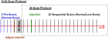
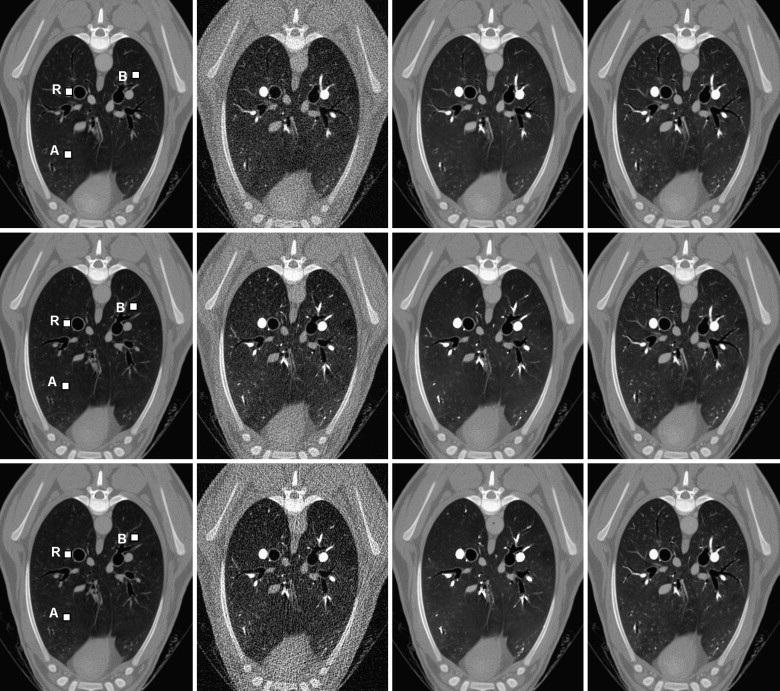
A sequence of sheep lung scans were performed in three prone, anesthetized sheep at normal and ultra-low doses. A scan protocol was developed for the ultra-low-dose studies with electrocardiographic gating: time point 1 for a normal x-ray dose scan (100 kV, 150 mAs) and time points 2 to 21 for low-dose scans (80 kV, 17 mAs). A nonlinear diffusion-based post-filtering method was applied to the difference images between the low-dose images and the high-quality reference image. The final images at 20 time points were generated by fusing the reference image with the filtered difference images.
Results
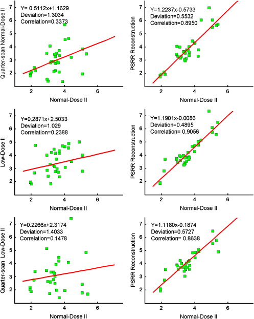
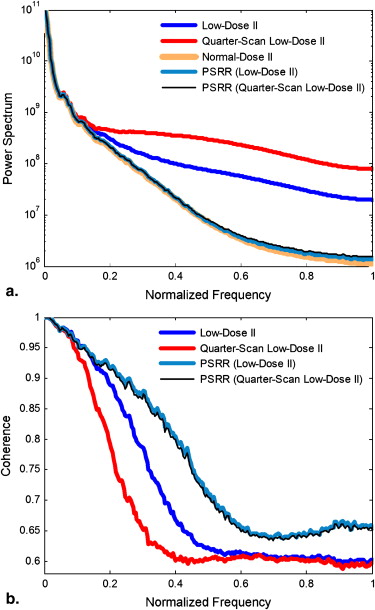
The power spectra of perfusion images and coherences in the normal scans showed a great improvement in image quality of the ultra-low-dose scans with PSRR relative to those without RSRR. The gamma variate fitting and the repeatability of the measurements of the mean transit time demonstrated that the key parameters of lung functions can be reliably accessed using PSRR. The variability of the ultra-low-dose scan results obtained using PSRR was not substantially different from that between two normal-dose scans.
Conclusions
This study demonstrates that an approximate 90% reduction in radiation dose is achievable using PSRR without compromising quantitative computed tomographic measurements of regional lung function.
Concern is growing worldwide about radiation-induced genetic, cancerous, and other diseases . Computed tomography is considered a radiation-intensive procedure, but it is becoming more and more common. In the mid-1990s, computed tomographic (CT) scans accounted for only 4% of total x-ray procedures, but they contributed 40% of the collective dose . With the introduction of helical, multislice, and cone-beam technologies, the use of computed tomography continues to increase. In the United States, the number of CT examinations performed has been estimated to be as high as nearly 60 million, accounting for 15% of imaging procedures and 75% of radiation exposure in 2002 . As many as 30% of patients undergoing one CT scan will have a total of at least three examinations, and >90% of abdominal or pelvic CT studies use two or more scans . A British study quantified the cancer risk from diagnostic x-rays, in which radiation from medical and dental scans is believed to cause about 700 cases of cancer per year in Britain and >5600 cases in the United States . On June 19, 2007, the New York Times reported that “the per-capita dose of ionizing radiation from clinical imaging exams in the U.S. increased almost 600% from 1980 to 2006.” More recently, in a high-profile article on the rapid growth in computed tomography and its associated radiation risks, Brenner and Hall estimated that “on the basis of such risk estimates and data on CT use from 1991 through 1996, it was estimated that about 0.4% of all cancers in the United States may be attributable to the radiation from CT studies. By adjusting this estimate for current CT use, this estimate might now be in the range of 1.5 to 2.0%.”
In the face of this increasing radiation risk, the well-known principle of “as low as reasonably achievable” is widely accepted in the medical community. Eliminating unnecessary CT examinations and optimizing CT protocols are important steps in minimizing radiation exposure, and a number of dose reduction techniques have been developed. These include methods to reduce milliampere-seconds, tube current modulation approaches , and a highly constrained back-projection reconstruction method . The operator-specified reduction of milliampere-seconds for small patients is prone to errors, which could conceivably increase patient dose if a study is repeated. More important, radiologists dislike computed tomography images with increased noise due to reduced milliampere-seconds. The tube current modulation approach uses information from either a scout view or a current scan view to change tube current dynamically during a scan, reducing the milliampere-seconds for thin body sections and increasing milliampere-seconds for thick sections. This strategy allows dose reductions of up to 30% to 40% for typical elliptical body sections. However, the gain diminishes for circular body sections. The highly constrained back-projection method is a new technique for the reconstruction of sparse, highly undersampled, time-resolved image data. This method originally was developed for magnetic resonance imaging and has been adapted for computed tomography . To the best of our knowledge, all current low-dose algorithms were developed to extract as much information as possible only from a low-dose data set of a patient or an animal , without the use of detailed prior knowledge from a previous scan of the same patient or animal.
Get Radiology Tree app to read full this article<
Get Radiology Tree app to read full this article<
Methods
Algorithm Description
Get Radiology Tree app to read full this article<

Get Radiology Tree app to read full this article<
Image Reconstruction
Get Radiology Tree app to read full this article<
Image Registration
Get Radiology Tree app to read full this article<
Nonlinear Filtering
Get Radiology Tree app to read full this article<
Get Radiology Tree app to read full this article<
Get Radiology Tree app to read full this article<
Image Registration
Get Radiology Tree app to read full this article<
Get Radiology Tree app to read full this article<
Nonlinear Filtering
Get Radiology Tree app to read full this article<
Get Radiology Tree app to read full this article<
∂u(x,t)/∂t=∇⋅[cd(x,t)∇u(x,t)], ∂
u
(
x
,
t
)
/
∂
t
=
∇
⋅
[
c
d
(
x
,
t
)
∇
u
(
x
,
t
)
]
,
where c d ( x , t ) is the diffusion conductance or diffusivity of the equation, and ∇ ∇ and ∇⋅ ∇
⋅ are respectively the gradient and divergence operators with respect to x . The solution of the above PDE leads to a filtered image. A key step of the PDE-based denoising is to choose an appropriate function c d . There are various choices for c d in different applications . If c d is a constant, Equation 1 becomes a linear diffusion equation. In this case, all the pixels including the edges are smoothed equally. If c d is image dependent, it becomes a nonlinear diffusion equation. Using a function c d constructed on the basis of the derivative of the image at time t , Perona and Malik were able to control the diffusion near the edges in the image. Note that in the difference image I D ( x ), we need to keep the features of high absolute gray levels and suppress interference of low absolute gray levels. Hence, we should construct a general c d on the basis of the image gray level and derivative at time t .
Get Radiology Tree app to read full this article<
Get Radiology Tree app to read full this article<
cd(x,t)={11−exp{−Cq[|∇uσ(x,t)|/λ]q{if|∇uσ(x,t)|=0if|∇uσ(x,t)|>0, c
d
(
x
,
t
)
=
{
1
if
|
∇
u
σ
(
x
,
t
)
|
=
0
1
−
exp
{
−
C
q
[
|
∇
u
σ
(
x
,
t
)
|
/
λ
]
q
{
if
|
∇
u
σ
(
x
,
t
)
|
0
,
where the contrast parameter λ defines diffusivity strength, constant parameter q > 1 defines the diffusivity change, and u σ ( x , t ) is the convolution of the current image u ( x , t ) with a Gaussian kernel of standard deviation σ. Letting g=|∇uσ(x,t)| g
=
|
∇
u
σ
(
x
,
t
)
| , we can calculate the dependent constant C q to make the flux g×{1−exp[−Cq(g/λ)q]} g
×
{
1
−
exp
[
−
C
q
(
g
/
λ
)
q
]
} ascending for g < λ and descending for g > λ. That is, C q is the solution of a nonlinear equation 1 − e − x − qxe − x = 0. Once the diffusivity c d ( x , t ) is determined, u ( x , t ) can be iteratively computed to arrive at a stable solution.
Get Radiology Tree app to read full this article<
Algorithm Implementation
Get Radiology Tree app to read full this article<
u(x,tp+1)=u(x,tp)+T{∇⋅[cd(x,tp)∇u(x,tp)]}, u
(
x
,
t
p
+
1
)
=
u
(
x
,
t
p
)
+
T
{
∇
⋅
[
c
d
(
x
,
t
p
)
∇
u
(
x
,
t
p
)
]
}
,
Get Radiology Tree app to read full this article<
Get Radiology Tree app to read full this article<
Table 1
The Values of λ and σ for the Iterative Procedure
p 0 1 2 3 4 5 λ 0.17 0.21 0.26 0.30 0.30 0.30 σ 2.00 1.50 1.00 0.50 0.50 0.50
Get Radiology Tree app to read full this article<
Results
Sheep Lung Perfusion Experiments
Get Radiology Tree app to read full this article<
Table 2
Key Parameters for the Sheep Perfusion Experiments
Study kVp mAs No. of Scans CTDI vol (mGy) Relative Dose Normal-dose I 100 150 20 108.77 100% Low-dose I 100 17 5 + 20 17.90 ∗ 16.5% Low-dose II 80 17 5 + 20 11.89 ∗ 10.9% Normal-dose II 100 150 20 108.77 100%
CTDI, computed tomography dose index.
Get Radiology Tree app to read full this article<
Get Radiology Tree app to read full this article<
Get Radiology Tree app to read full this article<
Get Radiology Tree app to read full this article<
PSRR Performance Analysis
Get Radiology Tree app to read full this article<
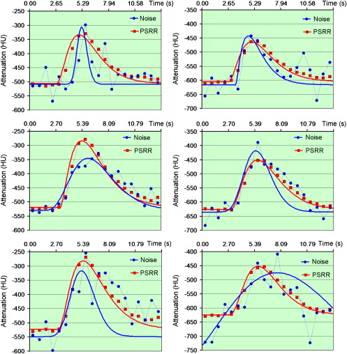
h(t)={A(t−t0)αexp[−(t−t0)/β]+h0h0t>t0t≤t0, h
(
t
)
=
{
A
(
t
−
t
0
)
α
exp
[
−
(
t
−
t
0
)
/
β
]
+
h
0
t
t
0
h
0
t
≤
t
0
,
where t is the independent time variable, t 0 is delay time, h 0 is the reference CT number, and A , α, and β are free parameters . As shown in Figure 7 , the gamma variate functions fitted from the CT numbers of the reconstructed PSRR images were better than their counterparts without PSRR.
Get Radiology Tree app to read full this article<
Get Radiology Tree app to read full this article<
Get Radiology Tree app to read full this article<
Get Radiology Tree app to read full this article<
Get Radiology Tree app to read full this article<
Discussion
Get Radiology Tree app to read full this article<
Get Radiology Tree app to read full this article<
Conclusion
Get Radiology Tree app to read full this article<
Acknowledgment
Get Radiology Tree app to read full this article<
Appendix
Power spectrum and coherence
Get Radiology Tree app to read full this article<
PN(wl,tk)=∑max{|um|,|vn|}=wlPI(um,vn,tk), P
N
(
w
l
,
t
k
)
=
∑
max
{
|
u
m
|
,
|
v
n
|
}
=
w
l
P
I
(
u
m
,
v
n
,
t
k
)
,
PL(wl,tk)=∑max{|um|,|vn|}=wlPL(um,vn,tk), P
L
(
w
l
,
t
k
)
=
∑
max
{
|
u
m
|
,
|
v
n
|
}
=
w
l
P
L
(
u
m
,
v
n
,
t
k
)
,
and
PNL(wl,tk)=∑max{|um|,|vn|}=wlPNL(um,vn,tk). P
NL
(
w
l
,
t
k
)
=
∑
max
{
|
u
m
|
,
|
v
n
|
}
=
w
l
P
NL
(
u
m
,
v
n
,
t
k
)
.
The final power spectra P¯¯¯N(wl) P
¯
N
(
w
l
) , P¯¯¯L(wl) P
¯
L
(
w
l
) , and P¯¯¯NL(wl) P
¯
NL
(
w
l
) are, respectively, the corresponding averages of P N ( w l , t k ), P L ( w l , t k ), and P NL ( w l , t k ) over time. Finally, the coherence is determined as
CNL(wl)=[P¯¯¯NL(wl)]2P¯¯¯N(wl)P¯¯¯L(wl), C
NL
(
w
l
)
=
[
P
¯
NL
(
w
l
)
]
2
P
¯
N
(
w
l
)
P
¯
L
(
w
l
)
,
which is a normalized coefficient.
Get Radiology Tree app to read full this article<
References
1. Brenner D., Elliston C., Hall E., Berdon W.: Estimated risks of radiation-induced fatal cancer from pediatric CT. AJR Am J Roentgenol 2001; 176: pp. 289-296.
2. Berrington de González A., Darby S.: Risk of cancer from diagnostic x-rays: estimates for the UK and 14 other countries. Lancet 2004; 363: pp. 345-351.
3. Brenner D.J., Hall E.J.: Computed tomography—an increasing source of radiation exposure. N Engl J Med 2007; 357: pp. 2277-2284.
4. Linton O.W., Mattler F.A.: National conference on dose reduction in computed tomography, emphasis on pediatrics. AJR Am J Roentgenol 2003; 181: pp. 321-329.
5. Mettler F.A., Wiest P.W., Locken J.A., Kelsey C.A.: CT scanning: patterns of use and dose. J Radiat Protect 2000; 20: pp. 353-359.
6. Jakobs T.F., Becker C.R., Ohnesorge B., et. al.: Multislice helical CT of the heart with retrospective ECG gating: reduction of radiation exposure by ECG-controlled tube current modulation. Eur Radiol 2002; 12: pp. 1081-1086.
7. Goo H.W., Suh D.S.: Tube current reduction in pediatric non-ECG-gated heart CT by combined tube current modulation. Pediatr Radiol 2006; 36: pp. 344-351.
8. O’Halloran R.L., Wen Z., Holmes J.H., Fain S.B.: Iterative projection reconstruction of time-resolved images using highly-constrained back-projection (HYPR). Magn Reson Med 2008; 59: pp. 132-139.
9. Supanich M., Rowley H., Turk A., Speidel M., Pulfer K., et. al.: An acquisition and image reconstruction scheme for reduced x-ray exposure dynamic 3D CTA. In: Medical imaging 2008: proceedings of SPIE. Bellingham, WA: SPIE 2008;
10. Carvalho B.A., Herman G.T.: Low-dose, large-angled cone-beam helical CT data reconstruction using algebraic reconstruction techniques. Image Vision Comput 2007; 25: pp. 78-94.
11. La Riviere P.J.: Penalized-likelihood sinogram smoothing for low-dose CT. Med Phys 2005; 32: pp. 1676-1683.
12. Wang G., Zhao S.Y., Heuscher D.: A knowledge-based cone-beam x-ray CT algorithm for dynamic volumetric cardiac imaging. Med Phys 2002; 29: pp. 1807-1822.
13. Kachelriess M., Kalender W.A.: Electrocardiogram-correlated image reconstruction from subsecond spiral computed tomography scans of the heart. Med Phys 1998; 25: pp. 2417-2431.
14. Noo F., Clackdoyle R., Pack J.D.: A two-step Hilbert transform method for 2D image reconstruction. Phys Med Biol 2004; 49: pp. 3903-3923.
15. Yu H., Wei Y., Hsieh J., Wang G.: Data consistency based translational motion artifact reduction in fan-beam CT. IEEE Trans Med Imaging 2006; 25: pp. 792-803.
16. Zitova B., Flusser J.: Image registration methods: a survey. Image Vision Comput 2003; 21: pp. 977-1000.
17. Hajnal J.V.Hill D.L.G.Hawkes D.J.Medical image registration.2001.CRC PressBoca Raton, FL:
18. Rohde G.K., Aldroubi A., Dawant B.M.: The adaptive bases algorithm for intensity-based nonrigid image registration. IEEE Trans Med Imaging 2003; 22: pp. 1470-1479.
19. Weeratunga S.K., Kamath C.: A comparison of PDE-based non-linear anistropic diffusion techniques for image denoising. Proc SPIE 2003; 5014: pp. 201-212.
20. Weeratunga S.K., Kamath C.: PDE-based non-linear diffusion techniques for denoising scientific and industrial images: an empirical study. Proc SPIE 2002; 4667: pp. 279-290.
21. Perona P., Malik J.: Scale-space and edge-detection using anisotropic diffusion. IEEE Trans Pattern Anal Machine Intell 1990; 12: pp. 629-639.
22. Madsen M.T.: A simplified formulation of the gamma variate function. Phys Med Biol 1992; 37: pp. 1597-1600.
23. Davenport R.: The derivation of the gamma-variate relationship for tracer dilution curves. J Nucl Med 1983; 24: pp. 945-948.
24. Won C., Chon D., Tajik J., et. al.: CT-based assessment of regional pulmonary microvascular blood flow parameters. J Appl Physiol 2003; 94: pp. 2483-2493.