
Rationale and Objectives
Computer-aided diagnosis (CAD) systems based on shape analysis have been proved to be highly accurate in evaluating breast tumors. However, it takes considerable time to train the classifier and diagnose breast tumors, because extracting morphologic features require a lot of computation. Hence, to develop a highly accurate and quick CAD system, we combined the texture and morphologic features of ultrasound breast tumor imaging to evaluate breast tumors in this study.
Materials and Methods
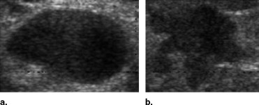
This study evaluated 210 ultrasound breast tumor images, including 120 benign tumors and 90 malignant tumors. The breast tumors were segmented automatically by the level set method. The autocovariance texture features and solidity morphologic feature were extracted, and a support vector machine was used to identify the tumor as benign or malignant.
Results
The accuracy of the proposed diagnostic system for classifying breast tumors was 92.86%, the sensitivity was 94.44%, the specificity was 91.67%, the positive predictive value was 89.47%, and the negative predictive value was 95.65%. In addition, the proposed system reduced the training time compared to systems based only on the morphologic analysis.
Conclusions
The CAD system based on texture and morphologic analysis can differentiate benign from malignant breast tumors with high accuracy and short training time. It is therefore clinically useful to reduce the number of biopsies of benign lesions and offer a second reading to assist inexperienced physicians in avoiding misdiagnosis.
Because of changing lifestyles and the polluted environment, the mortality rate for malignant tumors has had the highest rank of major causes of death in recent years. Breast cancer is the most common cancer in women. According to 2003 statistics, 211,300 women are expected to be diagnosed with this disease, and only lung cancer causes more death in women ( ). Because of such a high incidence, breast cancer must be studied.
To reduce the mortality rate and extend patients’ lives, early detection and prompt treatment for breast cancer are very important. Detection of breast cancer usually consists of physical examination, imaging, and biopsy ( ). Although biopsy is the best way to accurately determine whether a tumor is benign or malignant, it is invasive and costs much more than other detection methodologies. Moreover, most biopsies are avoidable because the probability of positive findings at biopsy for cancer is very low, between 10 and 31% ( ). To avoid unnecessary biopsy, many researchers have investigated computer-aided diagnosis (CAD) systems based on medical imaging ( ). The aim of these CAD systems is to offer more objective evidence and increase the physician’s diagnostic confidence.
Get Radiology Tree app to read full this article<
Get Radiology Tree app to read full this article<
Get Radiology Tree app to read full this article<
Materials and methods
Data Acquisition
Get Radiology Tree app to read full this article<
Get Radiology Tree app to read full this article<
Get Radiology Tree app to read full this article<
Feature Extraction
Get Radiology Tree app to read full this article<
Morphologic Features
Get Radiology Tree app to read full this article<
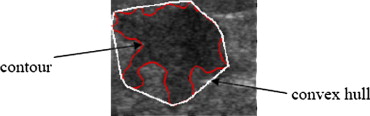
Solidity=Convex_Area−Area∑Ni=1Convex_Areai−Areai/N S
o
l
i
d
i
t
y
=
C
o
n
v
e
x
_
A
r
e
a
−
A
r
e
a
∑
i
=
1
N
C
o
n
v
e
x
_
A
r
e
a
i
−
A
r
e
a
i
/
N
where Area is the area of the tumor, Convex Area is the area of the convex hull of a tumor, and N is the number of tumors in the database. Figure 2 presents the convex hull of a tumor.
Get Radiology Tree app to read full this article<
Texture Features
Get Radiology Tree app to read full this article<
γ(Δm,Δn)=A(Δm,Δn)A(0,0). γ
(
Δ
m
,
Δ
n
)
=
A
(
Δ
m
,
Δ
n
)
A
(
0
,
0
)
.
We define Equation (3) as follows:
A(Δm,Δn)=1Count(Δm,Δn)⋅∑M−1−Δmx=0∑N−1−Δny=0[fin(x,y)−f¯in][fin(x+Δm,y+Δn)−f¯in] A
(
Δ
m
,
Δ
n
)
=
1
C
o
u
n
t
(
Δ
m
,
Δ
n
)
⋅
∑
x
=
0
M
−
1
−
Δ
m
∑
y
=
0
N
−
1
−
Δ
n
[
f
i
n
(
x
,
y
)
−
f
¯
in
]
[
f
i
n
(
x
+
Δ
m
,
y
+
Δ
n
)
−
f
¯
i
n
]
where fin(x,y) f
i
n
(
x
,
y
) and fin(x+Δm,y+Δn) f
i
n
(
x
+
Δ
m
,
y
+
Δ
n
) are the gray levels of two pixels inside a tumor, f¯in f
¯
i
n is the mean value of fin(x,y) f
i
n
(
x
,
y
) , and Count(Δm,Δn) C
o
u
n
t
(
Δ
m
,
Δ
n
) is the number of a pair of pixels that are both inside a tumor; distance along both the x and y axes between the two pixels is Δ m and Δ n , respectively.
Get Radiology Tree app to read full this article<
Get Radiology Tree app to read full this article<
Tumor Segmentation
Get Radiology Tree app to read full this article<
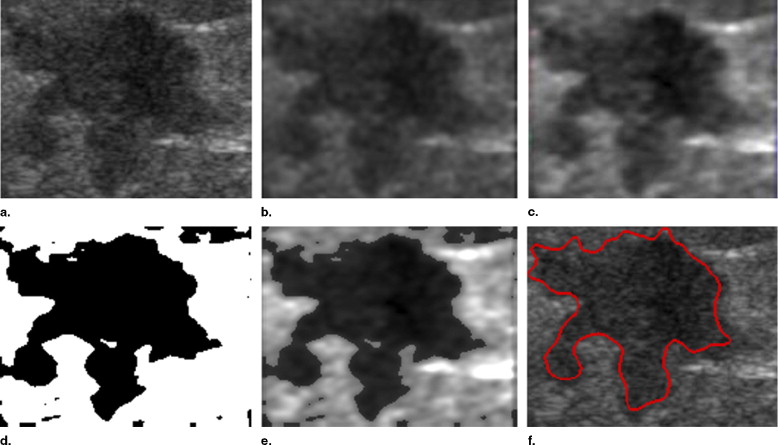
Anisotropic Diffusion Filtering
Get Radiology Tree app to read full this article<
Get Radiology Tree app to read full this article<
Stick Method
Get Radiology Tree app to read full this article<
Get Radiology Tree app to read full this article<
Automatic Threshold Method
Get Radiology Tree app to read full this article<
Level Set Method
Get Radiology Tree app to read full this article<
Get Radiology Tree app to read full this article<
Get Radiology Tree app to read full this article<
Get Radiology Tree app to read full this article<
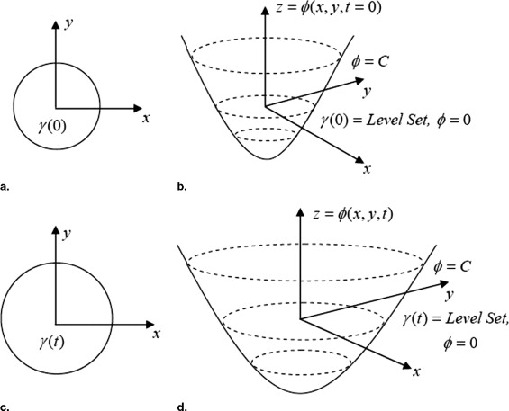
(x,t=0)=±d (
x
,
t
=
0
)
=
±
d
where d is the distance from x to γ(t=0) γ
(
t
=
0
) , and the sign is chosen if the point x is outside (plus) or inside (minus) the initial hypersurface γ(t=0) γ
(
t
=
0
) . Thus, we have an initial function (x,t=0):RN→R (
x
,
t
=
0
)
:
ℜ
N
→
ℜ with the property that
γ(t=0)=(x|(x,t=0)=0). γ
(
t
=
0
)
=
(
x
|
(
x
,
t
=
0
)
=
0
)
.
Get Radiology Tree app to read full this article<
Get Radiology Tree app to read full this article<
(x(t),t)=0. (
x
(
t
)
,
t
)
=
0.
Get Radiology Tree app to read full this article<
Get Radiology Tree app to read full this article<
t+∇(x(t),t)⋅x’(t)=0. t
+
∇
(
x
(
t
)
,
t
)
⋅
x
′
(
t
)
=
0.
Get Radiology Tree app to read full this article<
Get Radiology Tree app to read full this article<
t+F|∇|=0 t
+
F
|
∇
|
=
0
with a given value of (x,t=0) (
x
,
t
=
0
) . This is the level set equation introduced by Osher and Sethian ( ).
Get Radiology Tree app to read full this article<
Get Radiology Tree app to read full this article<
Get Radiology Tree app to read full this article<
Get Radiology Tree app to read full this article<
Get Radiology Tree app to read full this article<
Classifying with the SVM
Get Radiology Tree app to read full this article<
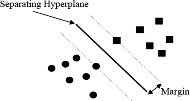
Get Radiology Tree app to read full this article<
Get Radiology Tree app to read full this article<
W(α)=∑Ni=1αi−12∑Ni,j=1αiαjyiyjΦ(xi)⋅Φ(xj) W
(
α
)
=
∑
i
=
1
N
α
i
−
1
2
∑
i
,
j
=
1
N
α
i
α
j
y
i
y
j
Φ
(x
i
)
⋅
Φ
(
x
j
)
where {(xi,yi),i=1,…,N} {
(
x
i
,
y
i
)
,
i
=
1
,
…
,
N
} is the training example set S , each example xi∈Rn x
i
∈
R
n belongs to a class labeled by yi∈{−1,1} y
i
∈
{
−
1
,
1
} , and Φ(x) Φ
(
x
) denotes a mapping function that maps x into a high-dimensional feature space. The corresponding training examples (xi,yi) (
x
i
,
y
i
) with nonzero coefficients α i are called support vectors.
Get Radiology Tree app to read full this article<
Get Radiology Tree app to read full this article<
W(α)=∑Ni=1αi−12∑Ni,j=1αiαjyiyjK(xi,xj) W
(
α
)
=
∑
i
=
1
N
α
i
−
1
2
∑
i
,
j
=
1
N
α
i
α
j
y
i
y
j
K
(
x
i
,x
j
)
where K is called a kernel function and must satisfy Mercer’s theorem ( ). Finally, the decision function becomes
f(x)=sgn(∑Ni=1αiyiK(xi,x)+b) f
(
x
)
=
sgn
(
∑
i
=
1
N
α
i
y
i
K
(
x
i
,
x
)
+
b
)
where b∈R b
∈
R is a constant.
Get Radiology Tree app to read full this article<
Get Radiology Tree app to read full this article<
Table 1
Four Common Types of Kernels Used in SVMs
Kernel typeK(xi,xj) K
(
x
i
,
x
j
) Linearx⋅z x
⋅
z Polynomial(γ⋅x⋅z+coef)d (
γ
⋅
x
⋅
z
+
c
o
e
f
)
d Gaussian radial basisexp(−γ⋅|x−z|2) exp
(
−
γ
⋅
|
x
−
z
|
2
) Sigmoidal neural networktanh(γ⋅x⋅z+coef) tanh
(
γ
⋅
x
⋅
z
+
c
o
e
f
)
Get Radiology Tree app to read full this article<
Results
Get Radiology Tree app to read full this article<
Get Radiology Tree app to read full this article<
Table 2
Classification of Breast Tumors by the Proposed Method
Sonographic classification Benign ⁎ Malignant ⁎ Benign TN 110 FN 5 Malignant FP 10 TP 85 Total 120 90
TP, true positive; TN, true negative; FP, false positive; FN, false negative.
Get Radiology Tree app to read full this article<
Get Radiology Tree app to read full this article<
Get Radiology Tree app to read full this article<
Table 3
Summary of Performance for Different Features
Item (a) (b) (c) (d) Accuracy 92.86% 88.57% 90.95% 83.33% Sensitivity 94.44% 85.56% 88.89% 85.56% Specificity 91.67% 90.83% 92.50% 81.67% PPV 89.47% 87.50% 89.89% 77.78% NPV 95.65% 89.34% 91.47% 88.29%
(a) The proposed method (combining morphological and texture features), (b) one morphological feature (which we used in the study), (c) six morphological features, and (d) texture features.
TP, true positive; TN, true negative; FP, false positive; FN, false negative.
Accuracy = (TP + TN)/(TP + TN + FP + FN)
Sensitivity = TP/(TP + FN)
Specificity = TN/(TN + FP)
Positive predictive value = TP/(TP + FP)
Negative predictive value = TN/(TN + FN)
Get Radiology Tree app to read full this article<
Get Radiology Tree app to read full this article<
Table 4
Time Comparison for Calculating Features of All Breast Tumor Images With Different Methods
Proposed method Morphologic Feature (one feature) Morphologic Features (six features) Time (sec) 112 66 812
Get Radiology Tree app to read full this article<
Discussion
Get Radiology Tree app to read full this article<
Get Radiology Tree app to read full this article<
Get Radiology Tree app to read full this article<
Get Radiology Tree app to read full this article<
References
1. Jemal A., Murray T., Samuels A., et. al.: Cancer statistics. CA Cancer J Clin 2003; 53: pp. 5-26.
2. Esserman L.J.: New approaches to the imaging, diagnosis, and biopsy of breast lesions. Cancer J 2002; 8: pp. S1-S14.
3. Bassett L.W., Liu T.H., Giuliano A.E., et. al.: The prevalence of carcinoma in palpable vs impalpable, mammographically detected lesions. AJR Am J Roentgenol 1991; 157: pp. 21-24.
4. Rubin M., Horiuchi K., Joy N., et. al.: Use of fine needle aspiration for solid breast lesions is accurate and cost-effective. Am J Surg 1997; 174: pp. 694-696.
5. Gisvold J.J., Martin J.K.: Prebiopsy localization of nonpalpable breast lesions. AJR Am J Roentgenol 1984; 143: pp. 477-481.
6. Palmedo H., Grunwald F., Bender H., et. al.: Scintimammography with technetium-99m methoxyisobutylisonitrile: Comparison with mammography and magnetic resonance imaging. Eur J Nucl Med 1996; 23: pp. 940-946.
7. Chang R.F., Wu W.J., Moon W.K., et. al.: Automatic ultrasound segmentation and morphology based diagnosis of solid breast tumors. Breast Cancer Res Treat 2005; 89: pp. 179-185.
8. Chen D.R., Chang R.F., Huang Y.L.: Computer-aided diagnosis applied to US of solid breast nodules by using neural networks. Radiology 1999; 213: pp. 407-412.
9. Stavros A.T., Thickman D., Rapp C.L., et. al.: Solid breast nodules: Use of sonography to distinguish between benign and malignant lesions. Radiology 1995; 196: pp. 123-134.
10. Chang R.F., Wu W.J., Moon W.K., et. al.: Support vector machines for diagnosis of breast tumors on US images. Acad Radiol 2003; 10: pp. 189-197.
11. Chang R.F., Wu W.J., Moon W.K., et. al.: Improvement in breast tumor discrimination by support vector machines and speckle-emphasis texture analysis. Ultrasound Med Biol 2003; 29: pp. 679-686.
12. Burges J.C.: A tutorial on support vector machines for pattern recognition. Data Mining Knowledge Discov 1998; 2: pp. 121-167.
13. Pontil M., Verri A.: Support vector machines for 3D object recognition. IEEE Trans Pattern Analy Machine Intell 1998; 20: pp. 637-646.
14. Vapnik V.N.: The Nature of Statistical Learning Theory.1995.Springer-VerlagNew York
15. Chapelle O., Haffner P., Vapnik V.N.: Support vector machines for histogram-based image classification. IEEE Trans Neural Networks 1999; 10: pp. 1055-1064.
16. Heiden V.D., Duin R.P.W., de Ridder D., et. al.: Classification, parameter estimation and state estimation: An engineering approach using MATLAB.2004.WileyOxford
17. Gerig G., Kubler O., Kikinis R., Jolesz F.A.: Nonlinear anisotropic filtering of MRI data. IEEE Trans Med Imaging 1992; 11: pp. 221-232.
18. Perona J., Malik J.: Scale-scape and edge-detection using anisotropic diffusion. IEEE Trans Pattern Analy Machine Intell 1990; 12: pp. 629-639.
19. Czerwinski R.N., Jones D.L., O’Brien W.D.: Edge detection in ultrasound speckle noise. IEEE Int Conf Image Processing 1994; 3: pp. 304-308.
20. Otsu N.: A threshold selection method form gray-level histograms. IEEE Trans Systems Man Cyber 1979; 9: pp. 62-66.
21. Sethian J.A.: Level Set Methods: Evolving Interfaces in Geometry, Fluid Mechanics, Computer Vision, and Materials Science.1996.Cambridge University PressCambridge
22. Osher S., Sethian J.: Fronts propagating with curvature-dependent speed: Algorithms based on Hamilton-Jacobi equations. J Comput Phys 1988; 79: pp. 12-49.