Using the Mean-to-Sigma Ratio as a Measure of the Improperness of Binormal ROC Curves

Rationale and Objectives

A basic assumption for a meaningful diagnostic decision variable is that there is a monotone relationship between the decision variable and the likelihood of disease. This relationship, however, generally does not hold for the binormal model. As a result, receiver operating characteristic (ROC)-curve estimation based on the binormal model produces improper ROC curves that are not concave over the entire domain and cross the chance line. Although in practice the “improperness” is typically not noticeable, there are situations where the improperness is evident. Presently, standard statistical software does not provide diagnostics for assessing the magnitude of the improperness.

Materials and Methods

We show how the mean-to-sigma ratio can be a useful, easy-to-understand and easy-to-use measure for assessing the magnitude of the improperness of a binormal ROC curve by showing how it is related to the chance-line crossing. We suggest an improperness criterion based on the mean-to-sigma ratio.

Results

Using a real-data example, we illustrate how the mean-to-sigma ratio can be used to assess the improperness of binormal ROC curves, compare the binormal method with an alternative proper method, and describe uncertainty in a fitted ROC curve with respect to improperness.

Conclusions

By providing a quantitative and easily computable improperness measure, the mean-to-sigma ratio provides an easy way to identify improper binormal ROC curves and facilitates comparison of analysis strategies according to improperness categories in simulation and real-data studies.

For diagnostic studies that evaluate and compare medical imaging modalities (eg, mammography) that require a human reader (typically a radiologist) to interpret generated images with respect to disease likelihood or severity, a commonly used method for estimating a receiver operating characteristic (ROC) curve is to use maximum likelihood estimation based on the assumption of a latent binormal model ; we refer to this method as the binormal method . The latent binormal model assumption states that there exists a monotone transformation that, when applied to the decision variable of interest, results in a latent decision variable that is normally distributed for nondiseased cases as well as for diseased cases, with the means and variances allowed to differ for the two distributions. For example, consider a study where a radiologist is asked to assign likelihood-of-disease confidence levels to images using a discrete five-level ordinal integer scale (eg, 1 = “definitely not diseased”, …, 5 = “definitely diseased”); for this situation, it is typical to assume that these ratings represent the binning of values of a latent (ie, unobserved) continuous decision variable representing the reader’s likelihood-of-disease perception. Often the ROC-curve summary measure of interest is the area under the curve (AUC).

For large samples, the binormal method has been shown to perform well for decision variable distributions that can vary greatly from the binormal distribution . We refer to the ROC curve corresponding to a latent binormal model decision variable as the binormal ROC curve . Throughout, we assume that the decision variable of interest is continuous and that larger values of it are more indicative of disease.

Get Radiology Tree app to read full this article<

Materials and methods

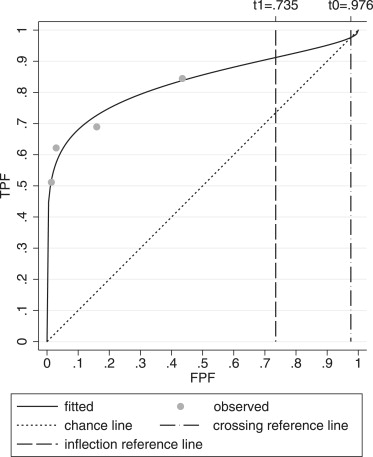
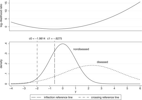
Example of a Noticeably Improper Binormal ROC Curve

Get Radiology Tree app to read full this article<

Table 1

Rating Data for a Radiologist from Van Dyke et al

Rating 1 2 3 4 5 Total Normal 39 19 9 1 1 69 Diseased 7 7 3 5 23 45

Get Radiology Tree app to read full this article<

Mean-to-Sigma Ratio as a Measure of Improperness

Get Radiology Tree app to read full this article<

r=μ2−μ1σ2−σ1 r

−

where μ 2 and σ 2 are the mean and standard deviation of the diseased latent decision variable distribution, and μ 1 and σ 1 are the corresponding parameters for the nondiseased latent decision variable distribution. Defining Δm = μ 2 − μ 1 and Δσ = σ 2 − σ 1 , we can write

r=ΔmΔσ r

Get Radiology Tree app to read full this article<

r=a1−b r

−

Get Radiology Tree app to read full this article<

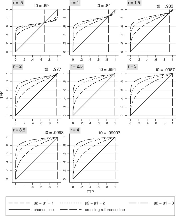
t0=Φ(r) t

(

)

with corresponding chance-line crossing threshold

c0=σ2μ1−σ1μ2σ2−σ1 c

−

Get Radiology Tree app to read full this article<

c0=−r c

−

Get Radiology Tree app to read full this article<

Table 2

Summary of Chance-line Crossing and Inflection-point Results for the Binormal Model with σ 1 ≠ σ 2

a) Chance-line crossing results fpf:t0=Φ(r) fpf:

(

) threshold:c0={σ2μ1−σ1μ2σ2−σ1−rgeneral formulaifμ1=0,σ1=1 threshold:

{

−

general formula

−

1 direction:{from above for increasing fpffrom below for increasing fpfifb<1ifb>1 direction:

{

from above for increasing fpf

from below for increasing fpf

1 b) Inflection-point results fpf:t1=Φ(σ1(μ2−μ1)σ22−σ21)=Φ(r1+b−1) fpf:

(

−

)

−

)

(

−

) threshold:c1=⎧⎩⎨⎪⎪−σ21μ2−σ22μ1σ22−σ21−μ2σ22−1=−r1+b−1general formulaifμ1=0,σ1=1 threshold:

{

−

general formula

−

1 Concave and convex segments of ROC curve:{concave over(0,t1)and convex over(t1,1)convex over(0,t1)and concave over(t1,1)ifb<1ifb>1 {

concave over

(

)

and convex over

(

)

convex over

(

)

and concave over

(

)

1 Slope of the likelihood and log-likelihood ratio functions:

⎧⎩⎨⎪⎪zeropositivenegativeifc=c1ifc>c1,b<1orc<c1,b>1ifc>c1,b>1orc<c1,b<1 {

zero

positive

negative

fpf, false-positive fraction; ROC, receiver operating characteristic.

The results are proved in the Appendix .

r = ( μ 2 − μ 1 )/( σ 2 − σ 1 ) is the mean-to-sigma ratio.

Get Radiology Tree app to read full this article<

Table 3

Mean-to-Sigma Ratio r and the Corresponding Chance-line Crossing fpf t 0 for the Binormal Model

r__t 0 −4.0 0.00003 −3.5 0.00023 −3.0 0.00135 −2.5 0.00621 −2.0 0.02275 −1.5 0.06681 −1.0 0.15866 −0.5 0.30854 0.0 0.50000 0.5 0.69146 1.0 0.84134 1.5 0.93319 2.0 0.97725 2.5 0.99379 3.0 0.99865 3.5 0.99977 4.0 0.99997

Get Radiology Tree app to read full this article<

σ2=σ1+(μ2−μ1)/r σ

(

−

)

Get Radiology Tree app to read full this article<

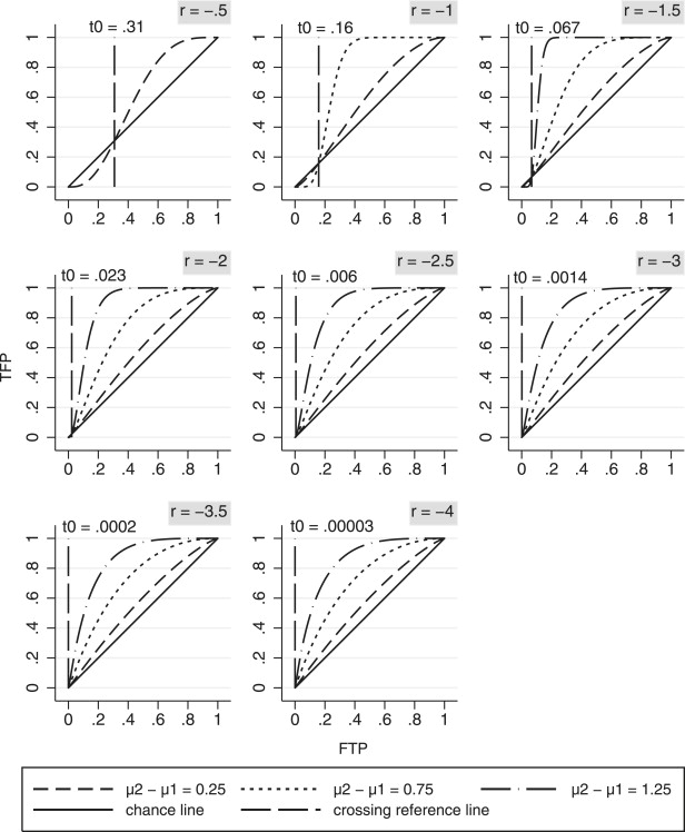
r=μ2−μ1σ1σ1σ2−σ1=μ2−μ1σ1b1−b r

−

shows that

|r|>(μ2−μ1)/σ1 |

(

−

)

for the Figure 4 combinations, because b > 1 and hence | b /(1− b )| > 1. Thus there is only one ROC curve in Figure 4 for r = −0.5, which corresponds to μ 2 − μ 1 = .25, since r cannot be equal to −.5 if μ 2 − μ 1 = .75 or μ 2 − μ 1 = 1.25 because of constraint . Similarly, there are only two curves in Figure 4 for r = −1.0 because r cannot be equal to −1.0 if μ 2 − μ 1 =1.25.

Get Radiology Tree app to read full this article<

Table 4

Improperness Classification of Binormal Receiver Operating Characteristic Curves Based on the Mean-to-Sigma Ratio r

Criteria Improperness Classification r | ≤ 2 Noticeable 2 < | r | < 3 Slight r | ≥ 3 Indiscernible

Get Radiology Tree app to read full this article<

Inflection-point fpf and Threshold

Get Radiology Tree app to read full this article<

t1=Φ(σ1(μ2−μ1)σ22−σ21)=Φ(r1+b−1) t

(

−

)

−

)

(

−

)

and the corresponding inflection-point threshold is given by

c1=−σ21μ2−σ22μ1σ22−σ21 c

−

Get Radiology Tree app to read full this article<

c1=−μ2σ22−1=−r1+b−1 c

−

Get Radiology Tree app to read full this article<

Proper Methods

Get Radiology Tree app to read full this article<

Improperness Classification Rule Proposed by Pan and Metz

Get Radiology Tree app to read full this article<

da|c|≤6 d

≤

with

da=2√a1+b2√andc=b−1b+1 d

and

−

where a and b are the binormal distribution parameters, and d a and c represent a parameterization of the corresponding binormal-LR model. (Actually, Metz and Pan use “ <∼ <

∼ ” instead of “≤”; we have substituted the latter symbol to facilitate comparison with r. ) We assume b ≠1 to avoid a zero denominator in d a /| c |. We show in the Appendix that

da|c|=|r|M d

where

M=2(b+1)21+b2−−−−−√ M

(

)

Get Radiology Tree app to read full this article<

|r|≤6/M |

≤

Get Radiology Tree app to read full this article<

M≤2 M

≤

with M = 2 if and only if b = 1. It follows from Eq. 12 and 13 that

if|r|<3thenda|c|≤6 if

then

≤

but the reverse implication does not hold; that is, our rule is more conservative in classifying a binormal curve as having an evident hook. For typical values of b , M is close to 2; in particular, if .5 ≤ b ≤ 2 then 1.90 ≤ M ≤ 2. For example, for b = 0.5 or 2.0, M = 1.90 and hence d a /| c | ≤ 6 if and only if | r | ≤ 3.16; more generally, for .5 ≤ b ≤ 2 the boundary of 6 in condition corresponds to a boundary between 3 and 3.16 for | r | for a given b . Thus we see that for typical values of b the boundary d a /| c | = 6 is similar to our proposed boundary of | r | = 3 separating slight and indiscernible improperness. On the other hand, if b = 0.1 or 10, then M = 1.548 and hence d a /| c | ≤ 6 if and only if | r | ≤ 3.88. For instance, if a = 3.0 and b = .1, then d a /| c | = 5.16 (from Eq. 11 ) and r = 3.33; here the hook should be evident according to rule but our rule says it is not evident, which we believe is a reasonable assertion since the chance line crossing occurs at the fpf value Φ(3.33)=.99957 Φ

(

3.33

)

.99957 . This last example illustrates an important advantage of the mean-to-sigma ratio – it has a clear interpretation of improperness in terms of the chance-line crossing.

Get Radiology Tree app to read full this article<

Simulation Study Implications

Get Radiology Tree app to read full this article<

Results

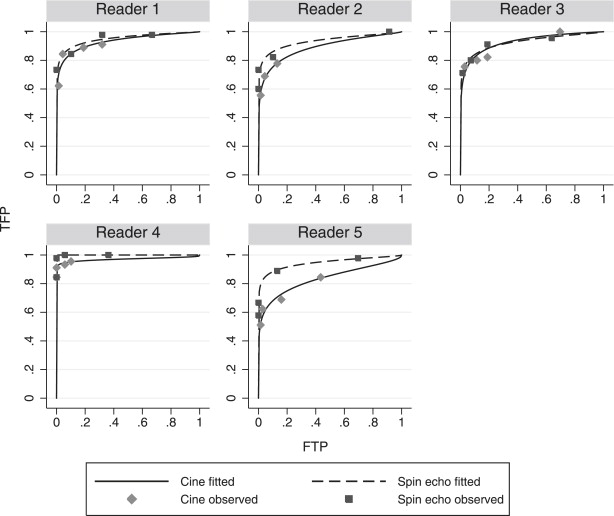
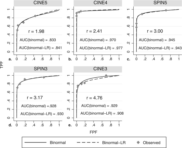
Example 1: Assessing the Degree of Improperness Using the Mean-to-Sigma Ratio

Get Radiology Tree app to read full this article<

Table 5

VanDyke et al Data Parameter Estimates

AUC r | Bootstrap Results Modality Reader_μ_ 2 σ 2 r__t 0 Binormal PROPROC Min 5th Percentile 95th Percentile Cine 1 3.17 1.86 3.67 0.9999 0.933 0.934 0.82 1.30 28.43 2 2.50 1.78 3.19 0.9993 0.890 0.891 0.53 0.88 29.41 3 2.74 1.58 4.76 1.0000 0.929 0.908 2.29 2.95 15.03 4 9.56 4.96 2.41 0.9921 0.970 0.977 1.00 1.43 16.45 5 2.29 2.16 1.98 0.9762 0.833 0.841 0.47 1.02 5.60 Spin echo 1 3.68 1.99 3.72 0.9999 0.951 0.952 1.33 1.95 42.69 2 3.70 2.24 2.99 0.9986 0.935 0.926 1.05 2.38 4.35 3 3.32 2.05 3.17 0.9992 0.928 0.930 1.17 1.68 17.57 4 6.93 1.21 33.19 1.0000 1.000 1.000 3.89 10.07 23.89 5 4.11 2.37 3.00 0.9986 0.945 0.943 1.32 1.82 8.04

All parameter estimates are based on the latent binormal model except for the PROPROC AUC (ie, the AUC for the binormal likelihood-ratio model estimated using the PROPROC procedure).

μ 2 and σ 2 are the mean and variance for the latent diseased distribution, μ 1 = 0 and σ 1 = 1 for the nondiseased distribution, r = ( μ 2 − μ 1 )/( σ 2 − σ 1 ) is the mean-to-sigma ratio, and t 0 = Φ (r) is the chance-line crossing fpf.

Minimum, 5th percentile, and 95th percentile are the minimum and 5th and 95th percentile values for | r | based on 1000 bootstrap samples.

Get Radiology Tree app to read full this article<

Example 2: Comparing the Binormal and Binormal-LR Methods Using the Mean-to-Sigma Ratio

Get Radiology Tree app to read full this article<

Example 3: Assessing Improperness Uncertainty

Get Radiology Tree app to read full this article<

Discussion

Get Radiology Tree app to read full this article<

Acknowledgments

Get Radiology Tree app to read full this article<

Supplementary data

Get Radiology Tree app to read full this article<

Appendix

Get Radiology Tree app to read full this article<

References

1. Dorfman D.D., Alf E.: Maximum likelihood estimation of parameters of signal-detection theory and determination of confidence intervals: rating method data. J Mathemat Psychol 1969; 6: pp. 487-496.
2. Dorfman D.D.: RSCORE II.Swets J.A.Pickett R.M.Evaluation of diagnostic systems: methods from signal detection theory.1982.Academic PressSan Diego, Calif:
3. Dorfman D.D., Berbaum K.S.: Degeneracy and discrete receiver operating characteristic rating data. Acad Radiol 1995; 2: pp. 907-915.
4. Metz C.E., Herman B.A., Shen J.H.: Maximum likelihood estimation of receiver operating characteristic (ROC) curves from continuously-distributed data. Stat Med 1998; 17: pp. 1033-1053.
5. Hanley J.A.: The robustness of the binormal assumptions used in fitting ROC curves. Med Decision Making 1988; 8: pp. 197-203.
6. Hanley J.A.: The use of the ‘binormal’ model for parametric ROC analysis of quantitative diagnostic tests. Stat Med 1996; 15: pp. 1575-1585.
7. HajianTilaki K.O., Hanley J.A., Joseph L., et. al.: A comparison of parametric and nonparametric approaches to ROC analysis of quantitative diagnostic tests. Med Decision Making 1997; 17: pp. 94-102.
8. Swets J.A.: Form of empirical ROCS in discrimination and diagnostic tasks: implications for theory and measurement of performance. Psychol Bull 1986; 99: pp. 181-198.
9. Pepe M.: The statistical evaluation of medical tests for classification and prediction.2003.Oxford University PressNew York
10. Egan J.P.: Signal detection theory and ROC analysis.1975.AcademicNew York
11. Stein S.K.: Calculus and analytic geometry.4th ed.1987.McGraw-HillNew York
12. Pan X.C., Metz C.E.: The ‘’proper’’ binormal model: parametric receiver operating characteristic curve estimation with degenerate data. Acad Radiol 1997; 4: pp. 380-389.
13. Van Dyke CW, White RD, Obuchowski NA, et al. Cine MRI in the diagnosis of thoracic aortic dissection. 79th RSNA Meetings, Chicago, Ill., November 28–December 3, 1993.
14. Swets J.A., Tanner W.P., Birdsall T.G.: Decision processes in perception. Psychol Rev 1961; 68: pp. 301-340.
15. Swets J.A.: Indices of discrimination or diagnostic accuracy: their ROCs and implied models. Psychol Bull 1986; 99: pp. 100-117.
16. Green D.M., Swets J.A.: Signal detection theory and psychophysics.1988.Peninsula PublishingLos Altos, Calif (Original work: Green DM, Swets JA. Signal detection theory and psychophysics. New York: Wiley, 1966.)
17. Dorfman D.D., Berbaum K.S., Metz C.E., et. al.: Proper receiver operating characteristic analysis: the bigamma model. Acad Radiol 1997; 4: pp. 138-149.
18. Dorfman D.D., Berbaum K.S., Brandser E.A.: A contaminated binormal model for ROC data—Part I. Some interesting examples of binormal degeneracy. Acad Radiol 2000; 7: pp. 420-426.
19. Dorfman D.D., Berbaum K.S.: A contaminated binormal model for ROC data—Part II. A formal model. Acad Radiol 2000; 7: pp. 427-437.
20. Dorfman D.D., Berbaum K.S.: A contaminated binormal model for ROC data—Part III. Initial evaluation with detection ROC data. Acad Radiol 2000; 7: pp. 438-447.
21. Metz C.E., Pan X.C.: “Proper” binormal ROC curves: theory and maximum-likelihood estimation. J Mathemat Psychol 1999; 43: pp. 1-33.
22. Hillis SL, Schartz KM, Pesce LL, et al. DBM MRMC procedure for SAS (computer software). Available for download from http://perception.radiology.uiowa.edu . Accessed August 1, 2009.
23. Berbaum KS, Schartz KM, Pesce LL, et al. DBM MRMC 2.2 (computer software). Available for download from http://perception.radiology.uiowa.edu . Accessed August 1, 2009.
24. Berbaum KS, Metz CE, Pesce LL, et al. DBM MRMC 2.1 User’s Guide (software manual). Available for download from http://perception.radiology.uiowa.edu . Accessed August 1, 2009.
25. Stein S.K.: Calculus in the first three dimensions.1967.McGraw-HillNew York

Using the Mean-to-Sigma Ratio as a Measure of the Improperness of Binormal ROC Curves

Rationale and Objectives

Materials and Methods

Results

Conclusions

Materials and methods

Example of a Noticeably Improper Binormal ROC Curve

Mean-to-Sigma Ratio as a Measure of Improperness

Inflection-point fpf and Threshold

Proper Methods

Improperness Classification Rule Proposed by Pan and Metz

Simulation Study Implications

Results

Example 1: Assessing the Degree of Improperness Using the Mean-to-Sigma Ratio

Example 2: Comparing the Binormal and Binormal-LR Methods Using the Mean-to-Sigma Ratio

Example 3: Assessing Improperness Uncertainty

Discussion

Acknowledgments

Supplementary data

References

Further Reading

A Preliminary Evaluation of Multi-probe Resonance-frequency Electrical Impedance Based Measurements of the Breast

An Ultrasound Model to Discriminate the Risk of Thyroid Carcinoma

Comparison of Chest Dual-energy Subtraction Digital Tomosynthesis Imaging and Dual-energy Subtraction Radiography to Detect Simulated Pulmonary Nodules with and without Calcifications