
Rationale and Objectives
The aim of this work was to validate and compare the statistical powers of proposed methods for analyzing free-response data using a search-model–based simulator.
Materials and Methods
A free-response data simulator is described that can model a single reader interpreting the same cases in two modalities, or two computer-aided detection (CAD) algorithms, or two human observers, interpreting the same cases in one modality. A variance components model, analogous to the Roe and Metz receiver-operating characteristic (ROC) data simulator, is described; it models intracase and intermodality correlations in free-response studies. Two generic observers were simulated: a quasi-human observer and a quasi-CAD algorithm. Null hypothesis (NH) validity and statistical powers of ROC, jackknife alternative free-response operating characteristic (JAFROC), a variant of JAFROC termed JAFROC-1, initial detection and candidate analysis (IDCA), and a nonparametric (NP) approach were investigated.
Results
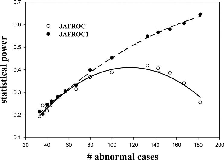
All methods had valid NH behavior over a wide range of simulator parameters. For equal numbers of normal and abnormal cases, for the human observer, the statistical power ranking of the methods was JAFROC-1 > JAFROC > (IDCA ∼ NP) > ROC. For the CAD algorithm, the ranking was (NP ∼ IDCA) > (JAFROC-1 ∼ JAFROC) > ROC. In either case, the statistical power of the highest ranked method exceeded that of the lowest ranked method by about a factor of two. Dependence of statistical power on simulator parameters followed expected trends. For data sets with more abnormal cases than normal cases, JAFROC-1 power significantly exceeded JAFROC power.
Conclusion
Based on this work, the recommendation is to use JAFROC-1 for human observers (including human observers with CAD assist) and the NP method for evaluating CAD algorithms.
Free-response data consist of mark-rating pairs ( ), classified into lesion localizations (LLs) or non-lesion localizations (NLs) according to their proximity to real lesions. The importance of assessing computer-aided detection (CAD) algorithms for mammography, low-dose computed tomographic (CT) screening for lung cancer, and other applications (eg, breast tomosynthesis, breast CT), has spurred renewed interest in methods for analyzing free-response data. Earlier methods ( ) assumed that the ratings of multiple marks on the same case were independent. This assumption drew criticism ( ) that discouraged usage, but end users of observer performance methodologies were faced with the dilemma of using questionable analyses or ignoring the location information and using receiver-operating characteristic (ROC) analysis instead. CAD algorithm evaluation for lung cancer screening presents this problem in an especially acute form. These algorithms generate tens of marks per image, and ignoring them is not a credible option. Fortunately, several new approaches to the analysis of free-response data are now available that do not depend on the independence assumption. However, these methods need to be validated and their statistical powers need to be compared.
Validation and statistical power studies are done via simulations that require a credible data simulator, or equivalently, a credible observer model. For example, the binormal model is widely used in the ROC context because it has had great success in fitting ROC data ( ). The search model ( ) is a candidate for a free-response data simulator. It is a mathematical parameterization of a perceptual model ( ) supported by eye-tracking measurements of how radiologists interpret images. The aims of this work were to develop a search model–based simulator and use the simulator to validate and compare the statistical powers of proposed methods for analyzing free-response data. The methods investigated were the jackknife alternative free-response operating characteristic (JAFROC) ( ), a variant of JAFROC termed JAFROC-1 ( ), initial detection and candidate analysis (IDCA) ( ), and a nonparametric (NP) method ( ). For comparison with an existing standard, the ROC method ( ) was also included.
Materials and methods
Get Radiology Tree app to read full this article<
The Search-model Simulator
Get Radiology Tree app to read full this article<
Get Radiology Tree app to read full this article<
nikt1∼Poi(λi). n
i
k
t
1
∼
P
o
i
(
λ
i
)
.
The number of signal-sites n ikt2 is realized by sampling a binomial random number generator with trial size N kt and probability of success ν i , where N kt is the number of lesions in case
nikt2∼binomial(Nkt,vi). n
i
k
t
2
∼
b
i
n
o
m
i
a
l
(
N
k
t
,
v
i
)
.
The notation allows for the possibility that λ and ν may depend on the modality, but a possible dependence of λ on case-truth is not considered in this work.
Get Radiology Tree app to read full this article<
Get Radiology Tree app to read full this article<
Get Radiology Tree app to read full this article<
ziktl1∼N(0,1), z
i
k
t
l
1
∼
N
(
0
,
1
)
,
ziktl2∼N(μi,1). z
i
k
t
l
2
∼
N
(
μ
i
,
1
)
.
For modality i, the simulator predicted FROC curve is defined by ( ):
NLFi(z)=λiΦ(−z) N
L
F
i
(
z
)
=
λ
i
Φ
(
−
z
)
LLFi(z)=viΦ(μi−z). L
L
F
i
(
z
)
=
v
i
Φ
(
μ
i
−
z
)
.
Intermodality and intracase correlations of the z iktls are modeled using a localization variance components method analogous to that developed for the ROC case ( ) by Roe and Metz (see Appendix ). ( F is the normal distribution function and F [ z ] = 1− F [ z ]).
Get Radiology Tree app to read full this article<
Simulated Observers
Get Radiology Tree app to read full this article<
Table 1
Simulation Parameters μ, λ, and ν for the Human Observer and CAD for the Two Modalities (1 and 2) and the Corresponding Areas (AUC 1 and AUC 2 ) under the Search Model–Predicted ROC Curves
Observer Modality 1 Modality 2 μ 1 λ 1 ν 1 AUC 1 μ 2 λ 2 ν 2 AUC 1 Human 1.50 1.3 0.80 0.80 1.55 1.04 0.88 0.85 CAD 2.34 10 0.90 2.37 8 0.99
AUC, area under the curve; CAD, computed-aided detection; ROC, receiver operating characteristic.
AUC 1 and AUC 2 were calculated numerically from the search model parameters ( ). These parameter values were used to generate the data in Tables 2–5 . Modality-1 parameters were chosen based on our experience with human observer and CAD-generated free-response receiver-operating characteristic curves. For a given AUC, the choice of search model parameters is not unique. The following rule was used to generate modality-2 parameters from those of modality-1: λ was 20% smaller. ν was 10% greater, and μ was adjusted to get the desired AUC value.
Get Radiology Tree app to read full this article<
Get Radiology Tree app to read full this article<
Get Radiology Tree app to read full this article<
Analysis of Free-response Data
Get Radiology Tree app to read full this article<
ROC
Get Radiology Tree app to read full this article<
JAFROC
Get Radiology Tree app to read full this article<
A′1=1NNNL∑NNi=1∑NLj=1ψ(Xi,Yj)ψ⎛⎝⎜X,Y⎞⎠⎟=⎡⎣⎢1.0ifY>X0.5ifY=X0.0ifY<X⎫⎭⎬⎪⎪⎪⎪⎪⎪⎪⎪. A
′
1
=
1
N
N
N
L
∑
i
=
1
N
N
∑
j
=
1
N
L
ψ
(
X
i
,
Y
j
)
ψ
(
X
,
Y
)
=
[
1.0
i
f
Y
X
0.5
i
f
Y
=
X
0.0
i
f
Y
<
X
}
.
X i is the ROC-equivalent rating for normal case i, Y j is the rating of the jth lesion, N N is the number of normal images, and N L is the number of lesions. The reason for the prime is because A′1 A
1
′ is the nonparametric estimate of the area under the alternative free-response receiver operating characteristic (AFROC) curve, previously denoted as A 1 ( ), except in JAFROC only normal images used to estimate the x-coordinate (ie, false-positive fraction) of the AFROC curve, whereas in the original definition all images are used. The AFROC curve is the plot of lesion localization fraction versus the false-positive fraction. The AFROC abscissa is identical to that of the ROC curve generated by the ROC-equivalent ratings ( ).
Get Radiology Tree app to read full this article<
JAFROC-1
Get Radiology Tree app to read full this article<
A1=1(NN+NA)NL∑NN+NAi=1∑NLj=1ψ(Xi,Yj). A
1
=
1
(
N
N
+
N
A
)
N
L
∑
i
=
1
N
N
+
N
A
∑
j
=
1
N
L
ψ
(
X
i
,
Y
j
)
.
Here, X i (i = N N+1 , N N +2, … , N N +N A ) is the highest NL rating on abnormal case i. Because it uses the highest rated NL on all images, JAFROC-1 is expected to have greater power than JAFROC. The difference is expected to be larger when the number of normal cases is small. In the limit of no normal cases, the JAFROC figure-of-merit, Equation 5 , cannot be calculated but that for JAFROC-1, Equation 6 , can.
Get Radiology Tree app to read full this article<
IDCA
Get Radiology Tree app to read full this article<
λ′=FNIv′=TNL}. λ
′
=
F
N
I
v
′
=
T
N
L
}
.
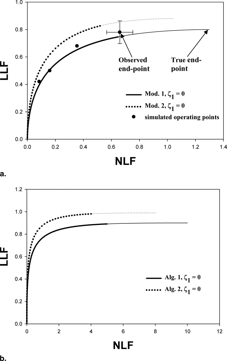
The primed notation is needed because the observed end point need not coincide with the simulator end point; for example, the observed end point in Figure 1 a, which is considerably to the left of the true end point at (1.3, 0.8). Under the binormal-model assumption, the z-samples for noise-sites are sampled from N(0,1) and z-samples for signal-sites are sampled from N(μ′,σ’2) N
(
μ
′
,
σ
′
2
) . The fitted FROC curve ( ) is:
NLF(z)=λ′Φ(−z)LLF(z)=v′Φ(μ′−zσ′)⎫⎭⎬. N
L
F
(
z
)
=
λ
′
Φ
(
−
z
)
L
L
F
(
z
)
=
v
′
Φ
(
μ
′
−
z
σ
′
)
}
.
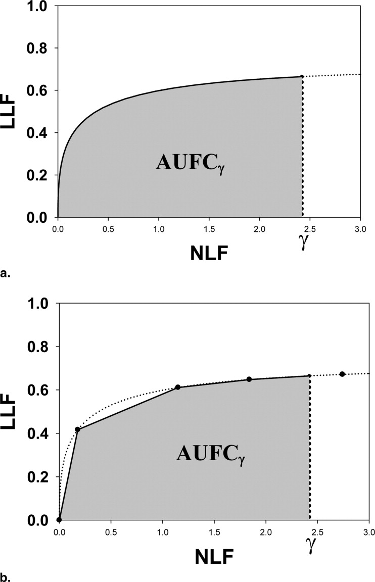
The parameters μ′ and σ′ were estimated by regarding the NL and LL marks as normal and abnormal “images” and fitting their ratings to the binormal model ( ) using the binormal model maximum likelihood program, whose output quantities, a and b, are related to μ′ and σ′ by μ′ = a/b and σ′ = 1/b. Alternatively “proper” ROC models may be used to fit the pseudo-ROC ( ). The fitted curve is referred to as a pseudo-ROC because the marks do not represent images; rather, they represent reported suspicious regions in the images (ie, parts of images). Note the fitted FROC curve is a scaled replica of the pseudo-ROC, with scaling factors λ′ and ν′ along the x and y axes, respectively, and that the fitted curved ends at the observed end point (this can be seen by setting z = −∞ in Eq 8 ) and cannot extend beyond it. The maximum-likelihood procedure requires the data to be binned. The binning ensured at least five counts in each of the two cells defined by adjacent cutoffs. For human observers, the number of bins was constrained to be ≤6 and the pseudo-ROC curve was fitted by the binormal model. For CAD, the number of bins was the maximum supported by the data subject to the limit that it be less than 20. The figure-of-merit ( ) was the partial area under the fitted FROC curve (AUFC) to the left of NLF = γ ( Fig 2 a) denoted by AUFC γ , which was evaluated by numerical integration of the curve predicted by Equation 8 .
Get Radiology Tree app to read full this article<
NP
Get Radiology Tree app to read full this article<
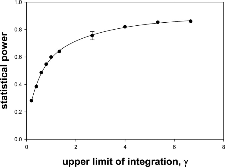
Choice of Upper Limit of Integration γ
Get Radiology Tree app to read full this article<
γ=λ2Φ(−ζ1)/1.2. γ
=
λ
2
Φ
(
−
ζ
1
)
/
1.2.
If the end point for any of the resampled datasets was to the left of this value, the simulation was repeated. This usually happened at the higher ζ 1 values and high correlations.
Get Radiology Tree app to read full this article<
Significance Testing
Get Radiology Tree app to read full this article<
Results
Get Radiology Tree app to read full this article<
Table 2
Null Hypothesis Rejection rates for the Human Observer for Different Conditions of Lowest Cutoff ζ 1 and Correlations ρ = ρ inter = ρ intra
ζ 1 and γ ρ Jackknife Bootstrap ROC JAFROC-1 JAFROC IDCA@γ NP@γ ζ 1 = −∞ γ = 0.867 0.1 0.0605 0.0513 0.0483 0.0500 0.0625 0.5 0.0565 0.0468 0.0495 0.0565 0.0660 0.9 0.0560 0.0528 0.0515 0.0640 0.0555 ζ 1 = −0.674 γ = 0.650 0.1 0.0435 0.0520 0.0460 0.0455 0.0465 0.5 0.0470 0.0565 0.0383 0.0505 0.0555 0.9 0.0495 0.0505 0.0573 0.0540 0.0485 ζ 1 = 0.0 γ = 0.433 0.1 0.0525 0.0480 0.0505 0.0480 0.0455 0.5 0.0560 0.0458 0.0473 0.0415 0.0620 0.9 0.0495 0.0560 0.0563 0.0505 0.0490 ζ 1 = 0.674 γ = 0.217 0.1 0.0520 0.0548 0.0525 0.0605 0.0480 0.5 0.0435 0.0448 0.0498 0.0555 0.0575 0.9 0.0495 0.0458 0.0443 0.0535 0.0470 Average 0.0513 0.0504 0.0493 0.0525 0.0536
AUC, area under the curve; IDCA, initial detection and candidate analysis; JAFROC, jackknife alternative free-response operating characteristic; NH, null hypothesis; NP, nonparametric; ROC, receiver operating characteristic.
The variable γ is the upper limit of integration for the area under the free response receiver-operating curve figure-of-merit, which applies to IDCA and NP methods only ( Eq 9 ). The simulation conditions were 100 normal cases, 100 abnormal cases, and 1 lesion per abnormal case; rejection rates were determined over 2000 simulations. The procedure used for significance testing is indicated in the top row. The search-model predicted AUCs for both modalities was 0.80. The last row is the average NH rejection rate over all conditions. Note that all methods had excellent NH behavior provided the appropriate method was used for significance testing. Use of the jackknife for the NP method gave poor NH behavior.
Table 3
NH Rejection Rates for the CAD Observer
ζ 1 and γ ρ Jackknife Bootstrap ROC JAFROC-1 JAFROC IDCA@γ NP@γ ζ 1 = −∞ γ = 6.67 0.1 0.0545 0.0498 0.0548 0.0495 0.0590 0.5 0.0590 0.0485 0.0455 0.0505 0.0630 0.9 0.0355 0.0405 0.0465 0.0460 0.0525 ζ 1 = −0.674 γ = 5 0.1 0.0475 0.0425 0.0510 0.0450 0.0500 0.5 0.0590 0.0480 0.0495 0.0550 0.0450 0.9 0.0550 0.0485 0.0463 0.0560 0.0600 ζ 1 = 0.0 γ = 3.33 0.1 0.0600 0.0565 0.0520 0.0520 0.0580 0.5 0.0470 0.0475 0.0488 0.0425 0.0595 0.9 0.0485 0.0525 0.0500 0.0550 0.0595 ζ 1 = 0.674 γ = 1.67 0.1 0.0480 0.0458 0.0430 0.0470 0.0515 0.5 0.0560 0.0568 0.0560 0.0590 0.0440 0.9 0.0480 0.0493 0.0470 0.0485 0.0445 Average 0.0515 0.0488 0.0492 0.0505 0.0539
AUC, area under the curve; CAD, computed-aided diagnosis; IDCA, initial detection and candidate analysis; JAFROC, jackknife alternative free-response operating characteristic; NH, null hypothesis; NP, nonparametric; ROC, receiver operating characteristic.
Other conditions are as in Table 2 . Note that all methods had excellent NH behavior.
Get Radiology Tree app to read full this article<
Get Radiology Tree app to read full this article<
Get Radiology Tree app to read full this article<
Table 4
Statistical Powers for the Human Observer for an Effect Size Δ(AUC) = 0.05
ζ 1 and γ ρ Jackknife Bootstrap ROC JAFROC-1 JAFROC IDCA@γ NP@γ ζ 1 = −∞ γ = 0.867 0.1 0.231 0.517 0.440 0.452 0.417 0.5 0.252 0.511 0.428 0.490 0.441 0.9 0.272 0.518 0.470 0.523 0.482 ζ 1 = −0.674 γ = 0.650 0.1 0.234 0.493 0.411 0.415 0.403 0.5 0.248 0.485 0.424 0.460 0.417 0.9 0.283 0.490 0.457 0.516 0.467 ζ 1 = 0.0 ⁎ γ = 0.433 ⁎ 0.1 0.224 0.440 0.397 0.349 0.319 0.5 0.242 0.453 0.377 0.393 0.390 0.9 0.282 0.495 0.448 0.417 0.402 ζ 1 = 0.674 ⁎ γ = 0.217 ⁎ 0.1 0.183 0.314 0.293 0.205 0.210 0.5 0.161 0.344 0.315 0.249 0.251 0.9 0.161 0.402 0.382 0.284 0.299 Average (all) 0.231 0.455 0.403 0.396 0.375 Average (*) 0.209 0.408 0.369 0.316 0.312
AUC, area under the curve; IDCA, initial detection and candidate analysis; JAFROC, jackknife alternative free-response operating characteristic; NP, nonparametric; ROC, receiver operating characteristic.
Other conditions are as in Table 2 . The next-to-last row is the power averaged over all 12 combinations of ρ and ζ 1 ; the last row is the power averaged over the rows relevant to human observers*. In either case, the ranking of the methods was JAFROC-1 > JAFROC > (IDCA ∼ NP) > ROC. The power of the highest ranked method (JAFROC-1) was almost twice that of the lowest ranked method (ROC).
Get Radiology Tree app to read full this article<
Table 5
Statistical Powers for the CAD Observer for an Effect Size Δ(AUC) = 0.05
ζ 1 and γ ρ Jackknife Bootstrap ROC JAFROC-1 JAFROC IDCA@γ NP@γ ζ 1 = −∞ ⁎ γ = 6.67 ⁎ 0.1 0.251 0.578 0.537 0.815 0.847 0.5 0.410 0.752 0.725 0.867 0.902 0.9 0.570 0.869 0.877 0.934 0.954 ζ 1 = −0.674 ⁎ γ = 5 ⁎ 0.1 0.244 0.569 0.538 0.801 0.799 0.5 0.366 0.764 0.727 0.858 0.859 0.9 0.584 0.878 0.880 0.924 0.945 ζ 1 = 0.0 γ = 3.33 0.1 0.239 0.600 0.559 0.700 0.712 0.5 0.375 0.734 0.717 0.787 0.807 0.9 0.616 0.879 0.873 0.919 0.952 ζ 1 = 0.674 γ = 1.67 0.1 0.233 0.558 0.522 0.554 0.530 0.5 0.380 0.660 0.647 0.666 0.629 0.9 0.574 0.828 0.811 0.835 0.853 Average (all) 0.403 0.722 0.701 0.805 0.816 Average ( ⁎ ) 0.404 0.735 0.714 0.866 0.884
AUC, area under the curve; CAD, computed-aided diagnosis; IDCA, initial detection and candidate analysis; JAFROC, jackknife alternative free-response operating characteristic; NP, nonparametric; ROC, receiver-operating characteristic.
Other conditions are as in Table 3 . The ranking of the methods was (NP ∼ IDCA) > (JAFROC-1 ∼ JAFROC) > ROC. The power of the highest ranked method (NP) is almost twice that of the lowest ranked method (ROC).
Get Radiology Tree app to read full this article<
Get Radiology Tree app to read full this article<
Get Radiology Tree app to read full this article<
Get Radiology Tree app to read full this article<
Get Radiology Tree app to read full this article<
Get Radiology Tree app to read full this article<
Get Radiology Tree app to read full this article<
Get Radiology Tree app to read full this article<
Discussion
Get Radiology Tree app to read full this article<
Get Radiology Tree app to read full this article<
Get Radiology Tree app to read full this article<
Get Radiology Tree app to read full this article<
Get Radiology Tree app to read full this article<
Acknowledgments
Get Radiology Tree app to read full this article<
Appendix
Variance Component Model for Free-response Tasks
Get Radiology Tree app to read full this article<
ziktls=μ0+Δμis+Ckt+(μC)ikt+(CL)ktls+(μCL)iktls. z
i
k
t
l
s
=
μ
0
+
Δ
μ
i
s
+
C
k
t
+
(
μ
C
)
i
k
t
+
(
C
L
)
k
t
l
s
+
(
μ
C
L
)
i
k
t
l
s
.
Because this is a one-reader model, the reader factor is absent. Because a location sample can only occur on a case, and not in isolation, terms such as L or μL are not included. Here (μ 0 + Δμ is ) represents the population average (over readers and cases) z-sample for a site with site-truth s in modality i and Δμ is is the modality effect that one is interested in detecting. Specifically, μ 0 = 0, μ 0 + Δμ 11 = 0, μ 0 + Δμ 12 = μ 1 , and μ 0 + Δμ 22 = μ 2 . The remaining terms in the equation represent independent and identically distributed samples from zero-mean Gaussian distributions with specified variances (the “variance components”) σ2C,σ2μC,σ2CL,andσ2μCL. σ
C
2
,
σ
μ
C
2
,
σ
C
L
2
,
a
n
d
σ
μ
C
L
2
. Specifically, Ckt∼N(0,σ2C) C
k
t
∼
N
(
0
,
σ
C
2
) is the contribution of
μ
C
)
i
k
t
∼
N
(
0
,
σ
μ
C
2
) is the contribution of
C
)
k
t
l
s
∼
N
(
0
,
σ
C
L
2
) is the contribution of site λs on
μ
C
L
)
i
k
t
l
s
∼
N
(
0
,
σ
μ
C
L
2
) is the contribution of site λs, on
μ
C
L
2 does not involve s), the variances are assumed to be independent of modality (no i-dependence), and correlations between signal sites and noise sites on the same case are neglected. There is a normalization constraint on the variance components associated with the case-factor and its interactions, namely:
σ2z≡VAR(zijktls)=σ2C+σ2μC+σ2LC+σ2μLC=1. σ
z
2
≡
V
A
R
(
z
i
j
k
t
l
s
)
=
σ
C
2
+
σ
μ
C
2
+
σ
L
C
2
+
σ
μ
L
C
2
=
1.
This ensures unit net variances of the signal- and noise-site samples, as required by the search-model simulator ( Eq 3a,b ).
Get Radiology Tree app to read full this article<
Correlation MM′_ LS_LS
Get Radiology Tree app to read full this article<
VAR(ziktls−zi′ktls)=VAR[{((μC)ikts+(μCL)iktls}−{(μC)i′kts+(μCL)i′ktls)}]VAR(ziktls−zi′ktls)=2σ2μC+2σ2μCL. V
A
R
(
z
i
k
t
l
s
−
z
i
′
k
t
l
s
)
=
V
A
R
[
{
(
(
μ
C
)
i
k
t
s
+
(
μ
C
L
)
i
k
t
l
s
}
−
{
(
μ
C
)
i
′
k
t
s
+
(
μ
C
L
)
i
′
k
t
l
s
)
}
]
V
A
R
(
z
i
k
t
l
s
−
z
i
′
k
t
l
s
)
=
2
σ
μ
C
2
+
2
σ
μ
C
L
2
.
Factors not shown on the right-hand side of the first of these equations are all fixed factors (μ, Δμ) because these do not contribute to the variance and factors that do not include modality (eg, C), because they cancel in the difference. The surviving factors are μC and μCL.
Get Radiology Tree app to read full this article<
Get Radiology Tree app to read full this article<
COR(x,y)=1−VAR(x−y)2VAR(y). C
O
R
(
x
,
y
)
=
1
−
V
A
R
(
x
−
y
)
2
V
A
R
(
y
)
.
Get Radiology Tree app to read full this article<
Get Radiology Tree app to read full this article<
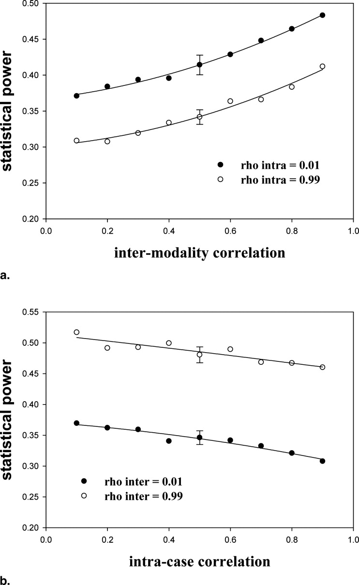
ρinter=COR(ziktls,zi’ktls)=σ2C+σ2CLσ2C+σ2μC+σ2CL+σ2μCL. ρ
inter
=
C
O
R
(
z
i
k
t
l
s
,
z
i
′
k
t
l
s
)
=
σ
C
2
+
σ
C
L
2
σ
C
2
+
σ
μ
C
2
+
σ
C
L
2
+
σ
μ
C
L
2
.
Get Radiology Tree app to read full this article<
Correlation MM_LS_L′S
Get Radiology Tree app to read full this article<
VAR(ziktls−ziktl’s)=VAR[{((CL)ktls+(μCL)iktls}−{((CL)ktl’s++(μCL)iktl’s}]VAR(ziktls−ziktl’s)=2σ2CL+2σ2μCL. V
A
R
(
z
i
k
t
l
s
−
z
i
k
t
l
′
s
)
=
V
A
R
[
{
(
(
C
L
)
k
t
l
s
+
(
μ
C
L
)
i
k
t
l
s
}
−
{
(
(
C
L
)
k
t
l
′
s
+
+
(
μ
C
L
)
i
k
t
l
′
s
}
]
V
A
R
(
z
i
k
t
l
s
−
z
i
k
t
l
′
s
)
=
2
σ
C
L
2
+
2
σ
μ
C
L
2
.
Get Radiology Tree app to read full this article<
Get Radiology Tree app to read full this article<
ρintra=COR(ziktls,ziktl’s)=σ2C+σ2μCσ2C+σ2μC+σ2CL+σ2μCL. ρ
intra
=
C
O
R
(
z
i
k
t
l
s
,
z
i
k
t
l
′
s
)
=
σ
C
2
+
σ
μ
C
2
σ
C
2
+
σ
μ
C
2
+
σ
C
L
2
+
σ
μ
C
L
2
.
Get Radiology Tree app to read full this article<
Determining the Variance Components from Specified Correlations
Get Radiology Tree app to read full this article<
Technical Details of the Simulator
Get Radiology Tree app to read full this article<
Get Radiology Tree app to read full this article<
References
1. Egan J.P., Greenburg G.Z., Schulman A.I.: Operating characteristics, signal detectability and the method of free response. J Acoust Soc Am 1961; 33: pp. 993-1007.
2. Bunch P.C., Hamilton J.F., Sanderson G.K., et. al.: A free-response approach to the measurement and characterization of radiographic-observer performance. J Appl Photogr Eng 1978; 4: pp. 166-171.
3. Chakraborty D.P.: Maximum Likelihood analysis of free-response receiver operating characteristic (FROC) data. Med Phys 1989; 16: pp. 561-568.
4. Chakraborty D.P., Winter L.H.L.: Free-response methodology: alternate analysis and a new observer-performance experiment. Radiology 1990; 174: pp. 873-881.
5. Swensson R.G.: Unified measurement of observer performance in detecting and localizing target objects on images. Med Phys 1996; 23: pp. 1709-1725.
6. Metz C.E.: Evaluation of digital mammography by ROC analysis.Doi K.Digital mammography ‘96.1996.Elsevier ScienceAmsterdam, The Netherlands:pp. 61-68.
7. Green D.M., Swets J.A.: Signal detection theory and psychophysics.1966.John Wiley & SonsNew York
8. Metz C.E.: Basic principles of ROC analysis. Semin Nucl Med 1978; 8: pp. 283-298.
9. Metz C.E.: ROC methodology in radiologic imaging. Invest Radiol 1986; 21: pp. 720-733.
10. Metz C.E.: Receiver operating characteristic analysis: a tool for the quantitative evaluation of observer performance and imaging systems. J Am Coll Radiol 2006; 3: pp. 413-422.
11. Chakraborty D.P.: ROC Curves predicted by a model of visual search. Phys Med Biol 2006; 51: pp. 3463-3482.
12. Chakraborty D.P.: A search model and figure of merit for observer data acquired according to the free-response paradigm. Phys Med Biol 2006; 51: pp. 3449-3462.
13. Yoon H.J., Zheng B., Sahiner B., et. al.: Evaluating computer-aided detection algorithms. Med Phys 2007; 34: pp. 2024-2038.
14. Kundel H.L., Nodine C.F.: A visual concept shapes image perception. Radiology 1983; 146: pp. 363-368.
15. Kundel H.L., Nodine C.F.: Modeling visual search during mammogram viewing. Proc SPIE 2004; 5372: pp. 110-115.
16. Kundel H.L., Nodine C.F., Conant E.F., et. al.: Holistic component of image perception in mammogram interpretation: gaze-tracking study. Radiology 2007; 242: pp. 396-402.
17. Chakraborty D.P., Berbaum K.S.: Observer studies involving detection and localization: modeling, analysis and validation. Med Phys 2004; 31: pp. 2313-2330.
18. Edwards D.C., Kupinski M.A., Metz C.E., et. al.: Maximum likelihood fitting of FROC curves under an initial-detection-and-candidate-analysis model. Med Phys 2002; 29: pp. 2861-2870.
19. Samuelson FW, Petrick N. Comparing image detection algorithms using resampling, 2006. IEEE International Symposium on Biomedical Imaging: From Nano to Micro 2006; 1312–1315.
20. Samuelson FW, Petrick N, Paquerault S. Advantages and examples of resampling for CAD evaluation. In: 2007 4th IEEE International Symposium on Biomedical Imaging: From Nano to Macro 2007; 492–495.
21. Dorfman D.D., Berbaum K.S., Metz C.E.: ROC characteristic rating analysis: generalization to the population of readers and patients with the jackknife method. Invest Radiol 1992; 27: pp. 723-731.
22. Chakraborty D.P., Yoon H.J.: Operating characteristics predicted by models for diagnostic tasks involving lesion localization. Med Phys 2008; 35: pp. 435-445.
23. Roe C.A., Metz C.E.: Dorfman-Berbaum-Metz method for statistical analysis of multireader, multimodality receiver operating characteristic data: validation with computer simulation. Acad Radiol 1997; 4: pp. 298-303.
24. Dorfman D.D., Alf E.: Maximum-likelihood estimation of parameters of signal-detection theory and determination of confidence intervals—rating-method data. J Math Psychol 1969; 6: pp. 487-496.
25. Eng J.: ROC analysis: web-based calculator for ROC curves. http://www.jrocfit.org Accessed May 27, 2008
26. Pan X., Metz C.E.: The proper binormal model: parametric receiver operating characteristic curve estimation with degenerate data. Acad Radiol 1997; 4: pp. 380-389.
27. Dorfman D.D., Berbaum K.S., Metz C.E., et. al.: Proper receiving operating characteristic analysis: the Bigamma model. Acad Radiol 1997; 4: pp. 138-149.
28. Metz C.E., Pan X.: Proper binormal ROC curves: theory and maximum-likelihood estimation. J Math Psychol 1999; 43: pp. 1-33.
29. Dorfman D.D., Berbaum K.S.: A contaminated binormal model for ROC data: part III. Acad Radiol 2000; 7: pp. 438-447.
30. Pesce L.L., Metz C.E.: Reliable and computationally efficient maximum-likelihood estimation of proper binormal ROC curves. Acad Radiol 2007; 14: pp. 814-829.
31. Efron B.: The jackknife, the bootstrap and other resampling plans.1982.Capital City PressMontpelier, VT
32. Zhou X.-H., Obuchowski N.A., McClish D.K.: Statistical methods in diagnostic medicine.2002.John Wiley & SonsNew York
33. Roe C.A., Metz C.E.: Variance-component modeling in the analysis of receiver operating characteristic index estimates. Acad Radiol 1997; 4: pp. 587-600.
34. Matsumoto M., Nishimura T.: Mersenne twister—a 623-dimensionally equidistributed uniform pseudorandom number generator. ACM Trans Model Comp Sim 1998; 8: pp. 3-30.
35. Galassi M., Davies J., Theiler J., et. al.: GNU scientific library reference manual.2005.Network Theory LimitedBristol, UK