
Rationale and Objectives
The purpose of this study was to develop a z -score mapping method on the basis of a voxel-by-voxel analysis to visualize hypoattenuation areas of hyperacute stroke on unenhanced computed tomographic (CT) images.
Materials and Methods
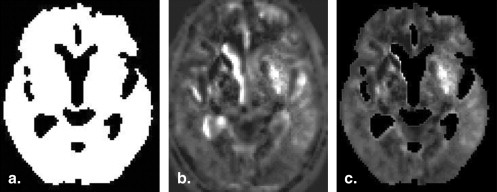
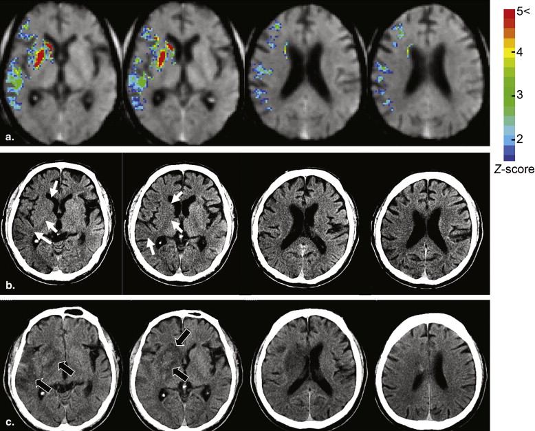
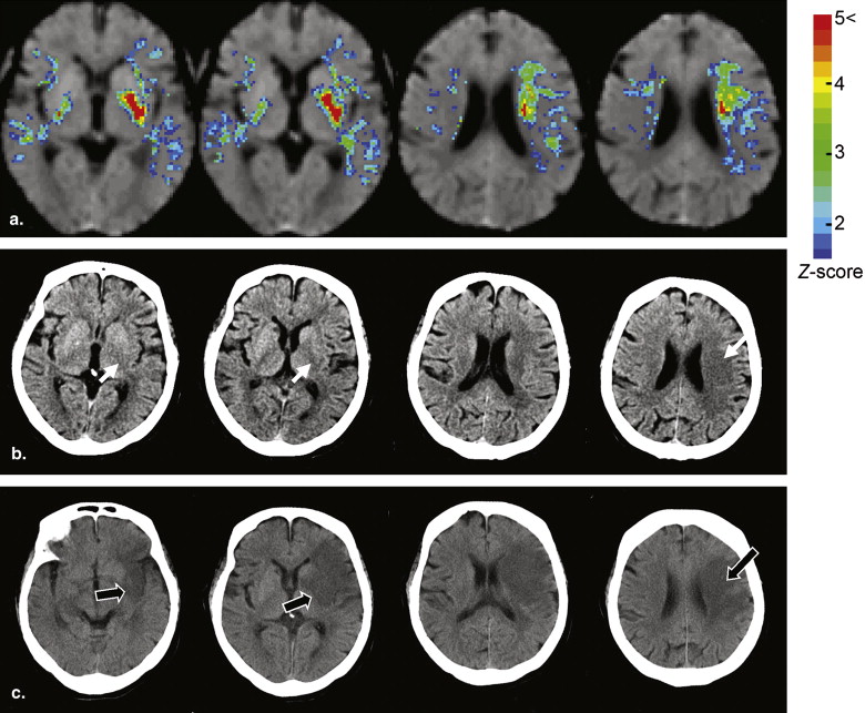
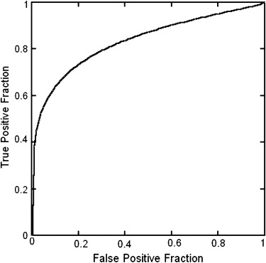
The algorithm of the developed method consisted of five main steps: anatomic standardization, the construction of a normal reference database, calculation of the z scores, the elimination of false-positive areas, and the extraction of hypoattenuation areas. The obtained z -score map was then superimposed on the original CT images for identifying hypoattenuation areas of hyperacute stroke on the unenhanced CT images. The method was applied to 21 patients with infarctions of the middle cerebral artery territory <3 hours after symptom onset. The performance of the method was evaluated using receiver-operating characteristic analysis.
Results
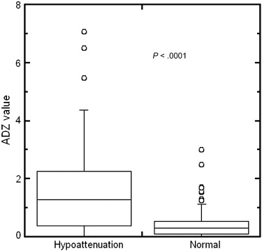
Hypoattenuation regions could be significantly distinguished from normal regions by z -score values ( P < .0001). The area under the receiver-operating characteristic curve for distinction between 68 hypoattenuation regions and 142 normal regions was 0.834.
Conclusions
The developed method has the potential to accurately indicate high–signal intensity areas corresponding to hypoattenuation areas on CT images in the hyperacute stage of stroke.
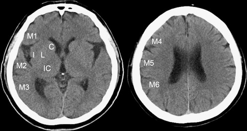
Currently, unenhanced computed tomographic (CT) imaging still serves as an initial neuroimaging examination in the diagnosis of acute ischemic stroke because of its accessibility and speed, although diffusion-weighted magnetic resonance (MR) imaging in acute ischemic stroke has been supported . Identifying hypoattenuation of ischemic brain parenchyma is important in the interpretation of acute stroke on CT images. Hypoattenuation is a subtle attenuation change (in Hounsfield units [HU]) of ischemic brain tissue. In recent years, tissue plasminogen activator thrombolysis has been approved by the US Food and Drug Administration as an effective treatment for acute stroke <3 hours after symptom onset. Patients with large areas of ischemic lesions would incur a high risk for fatal hemorrhagic complications after thrombolysis. To avoid the risk, unenhanced CT imaging plays an important role in rapidly selecting patients. Thus, quantifying the extent of areas of ischemic lesions is mandatory to select patients for thrombolysis with low risk for hemorrhage. A quantitative CT scoring system, the Alberta Stroke Program Early CT Score (ASPECTS) , is often used to help interpreters in quantifying the extent of ischemic lesions of acute stroke in the territory of the middle cerebral artery (MCA). When evaluating the extent of ischemic areas using the ASPECTS method, the extent of the regions of ischemic lesions (hypoattenuation or brain swelling) is quantified by counting the number of lesions among 10 predefined regions. However, the sensitivity for the detection of acute stroke was <50% on unenhanced CT images , even when the ASPECTS system was used.
The presence of hypoattenuation is an important CT finding of acute ischemic stroke. The detectability of hypoattenuation within a few hours of symptom onset largely depends on the skill and experiences of the reader, because of difficulty in the detection of subtle attenuation changes of ischemic brain tissue . Therefore, improvement in the detection of parenchymal hypoattenuation on unenhanced CT images would be desirable. To cope with this issue, we have developed an adaptive smoothing filter to reduce image noise . The results showed that the proposed filter had potential usefulness in the improvement of detection . However, the method was effective for detecting only the presence of hypoattenuation. The extent of hypoattenuation was difficult to identify with this method. Maldjian et al reported an automated segmentation method for identifying hypoattenuation of acute ischemia. In their report, histograms of voxel density distributions in the lentiform nucleus and insula were in comparison to those of the contralateral side on the brain image. The method, however, was limited to analyzing only two of the 10 regions in ASPECTS (ie, the lentiform nucleus and insula).
Get Radiology Tree app to read full this article<
Get Radiology Tree app to read full this article<
Materials and methods
Get Radiology Tree app to read full this article<
Get Radiology Tree app to read full this article<
Patient Database
Get Radiology Tree app to read full this article<
Get Radiology Tree app to read full this article<
Get Radiology Tree app to read full this article<
Get Radiology Tree app to read full this article<
Normalization
Get Radiology Tree app to read full this article<
Normal Reference Database
Get Radiology Tree app to read full this article<
Get Radiology Tree app to read full this article<
Calculation of z Score
Get Radiology Tree app to read full this article<
zscore(x,y,z)=[Cmean(x,y,z)− input(x,y,z)]/NSD(x,y,z), z
score
(
x
,
y
,
z
)
=
[
C
mean
(
x
,
y
,
z
)
− input
(
x
,
y
,
z
)
]
/
N
SD
(
x
,
y
,
z
)
,
where C mean( x , y , z ) and N SD( x , y , z ) represent the mean and SD, respectively of the normal reference data at the coordinate of ( x , y , z ). Input ( x , y , z ) is the value of spatially normalized patient data set at the same coordinate system. It is desirable that the z score in the area of normal brain parenchyma be nearly equal to zero. However, attenuation coefficients of the brain parenchyma on unenhanced CT images usually fluctuate because of variation in skull vault thickness. In this study, an offset was used to remove this variation during the calculation of z scores. The offset was the difference between an input CT value and the reference CT value. The determination of the offset was follows. First, two volumes of interest (VOIs) were determined from the mean data set. The two VOIs (size, 107 voxels), the right and left VOIs, were set at the right lentiform nucleus and the left lentiform nucleus, respectively. Second, the following measurements were made: the average value of the mean data set for the right VOI ( A R ) and that for the left VOI ( A L ) and the average value of the each input CT data set for the right VOI ( I R ) and that for the left VOI ( I L ). When measuring I R and I L , the VOIs were automatically set to each case of the input data. The offset value, V off , was defined as
Voff={AR−IRAL−ILwhenIR≥ILwhenIR<IL. V
of
f
=
{
A
R
−
I
R
A
L
−
I
L
when
I
R
≥
I
L
when
I
R
<
I
L
.
It is evident in equation 2 that the higher value of I R and I L was adopted for offsetting the input CT data set. The reason was that the VOI with the lower value relative to the contralateral VOI might include parenchymal hypoattenuation of acute stroke. After performing offsetting, the z score of each voxel of the input CT data was calculated using equation 1 .
Get Radiology Tree app to read full this article<
Elimination of Cerebrospinal Fluid (CSF) Area
Get Radiology Tree app to read full this article<
Get Radiology Tree app to read full this article<
Determination of the MCA Territory
Get Radiology Tree app to read full this article<
Display of z -score Maps
Get Radiology Tree app to read full this article<
Performance Evaluation
Get Radiology Tree app to read full this article<
Get Radiology Tree app to read full this article<
Results
Get Radiology Tree app to read full this article<
Get Radiology Tree app to read full this article<
Get Radiology Tree app to read full this article<
Get Radiology Tree app to read full this article<
Get Radiology Tree app to read full this article<
Get Radiology Tree app to read full this article<
Get Radiology Tree app to read full this article<
Discussion
Get Radiology Tree app to read full this article<
Get Radiology Tree app to read full this article<
Get Radiology Tree app to read full this article<
Get Radiology Tree app to read full this article<
Get Radiology Tree app to read full this article<
Get Radiology Tree app to read full this article<
Get Radiology Tree app to read full this article<
Conclusion
Get Radiology Tree app to read full this article<
Get Radiology Tree app to read full this article<
References
1. Adams H., Adams R., del Zoppo G.: Guidelines for the early management of patients with ischemic stroke: 2005 guidelines update a scientific statement from the Stroke Council of the American Heart Association/American Stroke Association. Stroke 2005; 36: pp. 916-923.
2. Adams J.H.P., Adams R.J., Brott T., et. al.: Guidelines for the early management of patients with ischemic stroke: a scientific statement from the Stroke Council of the American Stroke Association. Stroke 2003; 34: pp. 1056-1083.
3. Balbel P.A., Demchuk A.M., Zhang J., et. al.: Validity and reliability of a quantitative computed tomography score in predicting outcome of hyperacute stroke before thrombolytic therapy. Lancet 2000; 355: pp. 1670-1674.
4. Camargo E.C.S., Furie K.L., Singhal A.B., et. al.: Acute brain infarct: detection and delineation with CT angiographic source images versus nonenhanced CT scans. Radiology 2007; 244: pp. 541-548.
5. Schriger D.L., Karafut M., Starkman S., et. al.: Cranial computed tomography interpretation in acute stroke: physician accuracy in determining eligibility for thrombolytic therapy. JAMA 1998; 279: pp. 1293-1297.
6. Wardlaw J.M., Mielke O.: Early signs of brain infarction at CT: observer reliability and outcome after thrombolytic treatment—systematic review. Radiology 2005; 235: pp. 444-453.
7. Takahashi N., Lee Y., Tsai D.Y., et. al.: A novel noise reduction filter for improving visibility of early CT signs of hyperacute stroke: evaluation of the filter’s performance—preliminary clinical experience. Radiat Med 2007; 25: pp. 247-254.
8. Lee Y., Takahashi N., Tsai D.Y., et. al.: Adaptive partial median filter for early CT signs of acute cerebral infarction. Int J Comp Assisted Radiol Surg 2007; 2: pp. 105-115.
9. Takahashi N., Lee Y., Tsai D.Y., et. al.: Improvement of detection of hypoattenuation in acute ischemic stroke in unenhanced CT using an adaptive smoothing Filter. Acta Radiologica 2008; 49: pp. 816-826.
10. Maldjian J.A., Chalela J., Kasner S.E., et. al.: Automated CT segmentation and analysis for acute middle cerebral artery stroke. AJNR Am J Neuroradiol 2001; 22: pp. 1050-1055.
11. Minoshima S., Frey K.A.A., Koeppe R.A., et. al.: A diagnostic approach in Alzheimer’s disease using three-dimensional stereotactic surface projections of fluorine-18-FDG PET. J Nucl Med 1995; 36: pp. 1238-1248.
12. Matsuda H., Mizunuma S., Nagao T., et. al.: Automated discrimination between very early Alzheimer disease and controls using an easy Z-score imaging system for multicenter brain perfusion single-photon emission tomography. AJNR Am J Neuroradiol 2007; 28: pp. 731-736.
13. Friston K.J., Ashburner J., Frith C.D., et. al.: Spatial registration and normalization of images. Hum Brain Mapp 1995; 3: pp. 165-189.
14. Ashburner J., Friston K.J.: Nonlinear spatial normalization using basis functions. Hum Brain Mapp 1999; 7: pp. 254-266.